Page 439 - Matrix Analysis & Applied Linear Algebra

5.13 Orthogonal Projection 435

so, according to (5.13.4),

T
P R(A) = U 1 U = AA , P N(A T ) = I − P R(A) = I − AA ,
†
†
1
(5.13.12)
T
P R(A T ) = V 1 V = A A, P N(A) = I − P R(A T ) = I − A A.
†
†
1
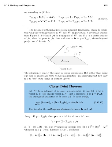
The notion of orthogonal projection in higher-dimensional spaces is consis-
3
2
tent with the visual geometry in and . In particular, it is visually evident
3
from Figure 5.13.4 that if M is a subspace of , and if b is a vector outside
of M, then the point in M that is closest to b is p = P M b, the orthogonal
projection of b onto M.
b
min b − m 2
m∈M
M
0 p = P M b

Figure 5.13.4
The situation is exactly the same in higher dimensions. But rather than using
our eyes to understand why, we use mathematics—it’s surprising just how easy
it is to “see” such things in abstract spaces.

Closest Point Theorem
Let M be a subspace of an inner-product space V, and let b be a
vector in V. The unique vector in M that is closest to b is p = P M b,
the orthogonal projection of b onto M. In other words,

min b − m = b − P M b = dist (b, M). (5.13.13)
2
2
m∈M
This is called the orthogonal distance between b and M.

Proof. If p = P M b, then p − m ∈M for all m ∈M, and

⊥
b − p =(I − P M )b ∈M ,
2 2 2
so (p − m) ⊥ (b − p). The Pythagorean theorem says x + y = x + y
whenever x ⊥ y (recall Exercise 5.4.14), and hence

2 2 2 2 2
b − m = b − p + p − m = b − p + p − m ≥ p − m .
2 2 2 2 2