Page 442 - Matrix Analysis & Applied Linear Algebra

438 Chapter 5 Norms, Inner Products, and Orthogonality

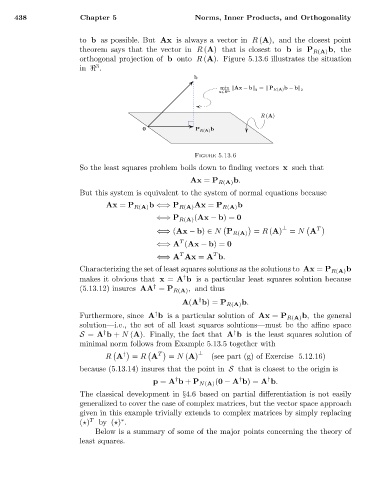
to b as possible. But Ax is always a vector in R (A), and the closest point
theorem says that the vector in R (A) that is closest to b is P R(A) b, the
orthogonal projection of b onto R (A). Figure 5.13.6 illustrates the situation
3
in .
b
min Ax − b = P R(A) b − b
x∈ n 2 2

R (A)
0 P R(A) b

Figure 5.13.6
So the least squares problem boils down to finding vectors x such that
Ax = P R(A) b.
But this system is equivalent to the system of normal equations because
Ax = P R(A) b ⇐⇒ P R(A) Ax = P R(A) b
⇐⇒ P R(A) (Ax − b)= 0
T
⊥
⇐⇒ (Ax − b) ∈ N P R(A) = R (A) = N A
T
⇐⇒ A (Ax − b)= 0
T
T
⇐⇒ A Ax = A b.
Characterizing the set of least squares solutions as the solutions to Ax = P R(A) b
makes it obvious that x = A b is a particular least squares solution because
†
†
(5.13.12) insures AA = P R(A) , and thus
A(A b)= P R(A) b.
†
Furthermore, since A b is a particular solution of Ax = P R(A) b, the general
†
solution—i.e., the set of all least squares solutions—must be the affine space
S = A b + N (A). Finally, the fact that A b is the least squares solution of
†
†
minimal norm follows from Example 5.13.5 together with
T
R A † = R A = N (A) ⊥ (see part (g) of Exercise 5.12.16)
because (5.13.14) insures that the point in S that is closest to the origin is
†
†
†
p = A b + P N(A) (0 − A b)= A b.
The classical development in §4.6 based on partial differentiation is not easily
generalized to cover the case of complex matrices, but the vector space approach
given in this example trivially extends to complex matrices by simply replacing
( ) T by ( ) .
∗
Below is a summary of some of the major points concerning the theory of
least squares.