Page 441 - Matrix Analysis & Applied Linear Algebra

5.13 Orthogonal Projection 437

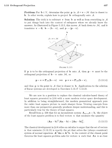
Problem: For b ∈V, determine the point p in A = v + M that is closest to
b. In other words, explain how to project b orthogonally onto A.
Solution: The trick is to subtract v from b as well as from everything in A
to put things back into the context of subspaces where we already know the
answers. As illustrated in Figure 5.13.5, this moves A back downto M, and it
translates v → 0, b → (b − v), and p → (p − v).

b

A = v + M
p
v b − v

M p - v
p − v
0
0

Figure 5.13.5
If p is to be the orthogonal projection of b onto A, then p − v must be the
orthogonal projection of b − v onto M, so

p − v = P M (b − v)=⇒ p = v + P M (b − v), (5.13.14)

and thus p is the point in A that is closest to b. Applications to the solution
of linear systems are developed in Exercises 5.13.17–5.13.22.

We are now in a position to replace the classical calculus-based theory of
least squares presented in §4.6 with a more modern vector space development.
In addition to being straightforward, the modern geometrical approach puts
the entire least squares picture in much sharper focus. Viewing concepts from
more than one perspective generally produces deeper understanding, and this is
particularly true for the theory of least squares.
Recall from p. 226 that for an inconsistent system A m×n x = b, the object
of the least squares problem is to find vectors x that minimize the quantity

2
T
(Ax − b) (Ax − b)= Ax − b . (5.13.15)
2
The classical development in §4.6 relies on calculus to argue that the set of vectors
x that minimize (5.13.15) is exactly the set that solves the (always consistent)
T
T
system of normal equations A Ax = A b. In the context of the closest point
theorem the least squares problem asks for vectors x such that Ax is as close