Page 447 - Matrix Analysis & Applied Linear Algebra

5.13 Orthogonal Projection 443

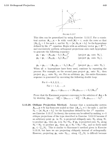
Figure 5.13.7
This idea can be generalized by using Exercise 5.13.17. For a consis-
tent system A n×r x = b with rank (A)= r, scale the rows so that
A i∗ =1 for each i, and let H i = {x | A i∗ x = b i } be the hyperplane
2
defined by the i th equation. Begin with an arbitrary vector p 0 ∈ r×1 ,
and successively perform orthogonal projections onto each hyperplane
to generate the following sequence:
T
p 1 = p 0 − (A 1∗ p 0 − b 1 )(A 1∗ ) (project p 0 onto H 1 ),
T
p 2 = p 1 − (A 2∗ p 1 − b 2 )(A 2∗ ) (project p 1 onto H 2 ),
. .
. .
. .
T
p n = p n−1 − (A n∗ p n−1 − b n )(A n∗ ) (project p n−1 onto H n ).
When all n hyperplanes have been used, continue by repeating the
process. For example, on the second pass project p n onto H 1 ; then
project p n+1 onto H 2 , etc. For an arbitrary p 0 , the entire Kaczmarz
sequence is generated by executing the following double loop:

For k =0, 1, 2, 3,...
For i =1, 2,...,n
T
p kn+i = p kn+i−1 − (A i∗ p kn+i−1 − b i )(A i∗ )
Prove that the Kaczmarz sequence converges to the solution of Ax = b
2 2 2
by showing p kn+i − x = p kn+i−1 − x − (A i∗ p kn+i−1 − b i ) .
2 2
5.13.20. Oblique Projection Method. Assume that a nonsingular system
A n×n x = b has been row scaled so that A i∗ =1 for each i, and let
2
H i = {x | A i∗ x = b i } be the hyperplane defined by the i th equation—
see Exercise 5.13.17. In theory, the system can be solved by making n−1
oblique projections of the type described in Exercise 5.13.18 because if
an arbitrary point p 1 in H 1 is projected obliquely onto H 2 along H 1
to produce p 2 , then p 2 is in H 1 ∩H 2 . If p 2 is projected onto H 3 along
H 1 ∩H 2 to produce p 3 , then p 3 ∈H 1 ∩H 2 ∩H 3 , and so forth until
n
p n ∈∩ H i . This is similar to Kaczmarz’s method given in Exercise
i=1
5.13.19, but here we are projecting obliquely instead of orthogonally.
k
However, projecting p k onto H k+1 along ∩ H i is difficult because
i=1