Page 452 - Matrix Analysis & Applied Linear Algebra
P. 452

448              Chapter 5                    Norms, Inner Products, and Orthogonality

                                    where ε i is a random variable accounting for the i th  observation (or mea-
                                                 63
                                    surement) error. It is generally valid to assume that observation errors are not
                                    correlated with each other but have a common variance (not necessarily known)
                                    and a zero mean. In other words, we assume that
                                                                                    2
                                                                                   σ   when i = j,
                                            E[ε i ]=0 for each i  and  Cov[ε i ,ε j ]=
                                                                                   0   when i  = j.
                                                                                                
                                             y 1          x 11  x 12  ···  x 1n         β 1         ε 1
                                            y 2        x 21  x 22  ···  x 2n      β 2        ε 2 
                                    If y =    .   , X =    .  .   .     .   , β =    .   , ε =    .   ,
                                              .             .    .     .   .            .            .
                                            .          .      .    .    .         .          . 
                                             y m          x m1  x m2  ··· x mn          β n         ε m
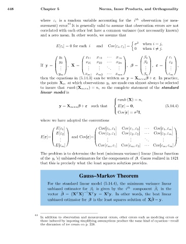
                                    then the equations in (5.14.3) can be written as y = X m×n β + ε. In practice,
                                    the points X i∗ at which observations y i are made can almost always be selected
                                    to insure that rank (X m×n )= n, so the complete statement of the standard
                                    linear model is
                                                                        
                                                                         rank (X)= n,
                                                                        
                                             y = X m×n β + ε such that    E[ε]= 0,                (5.14.4)
                                                                        
                                                                                   2
                                                                          Cov[ε]= σ I,
                                    where we have adopted the conventions
                                                                                                    
                                            E[ε 1 ]              Cov[ε 1 ,ε 1 ]  Cov[ε 1 ,ε 2 ]  ···  Cov[ε 1 ,ε m ]
                                                                Cov[ε 2 ,ε 1 ]  Cov[ε 2 ,ε 2 ]  ···
                                          E[ε 2 ]                                          Cov[ε 2 ,ε m ] 
                                    E[ε]=    .    and Cov[ε]=     .           .      .        .      .
                                             .                       .           .        .      .
                                            .                     .           .       .       .     
                                           E[ε m ]               Cov[ε m ,ε 1 ]Cov[ε m ,ε 2 ] ··· Cov[ε m ,ε m ]
                                    The problem is to determine the best (minimum variance) linear (linear function
                                    of the y i ’s) unbiased estimators for the components of β. Gauss realized in 1821
                                    that this is precisely what the least squares solution provides.


                                                       Gauss–Markov Theorem
                                       For the standard linear model (5.14.4), the minimum variance linear
                                                                                             ˆ
                                       unbiased estimator for β i is given by the i th  component β i in the

                                              ˆ
                                                             T
                                                      T
                                       vector β = X X      −1 X y = X y. In other words, the best linear
                                                                     †
                                                                                            ˆ
                                       unbiased estimator for β is the least squares solution of Xβ = y.
                                 63
                                    In addition to observation and measurement errors, other errors such as modeling errors or
                                    those induced by imposing simplifying assumptions produce the same kind of equation—recall
                                    the discussion of ice cream on p. 228.
   447   448   449   450   451   452   453   454   455   456   457