Page 448 - Matrix Analysis & Applied Linear Algebra

444 Chapter 5 Norms, Inner Products, and Orthogonality

k
∩ H i is generally unknown. This problem is overcome by modifying
i=1
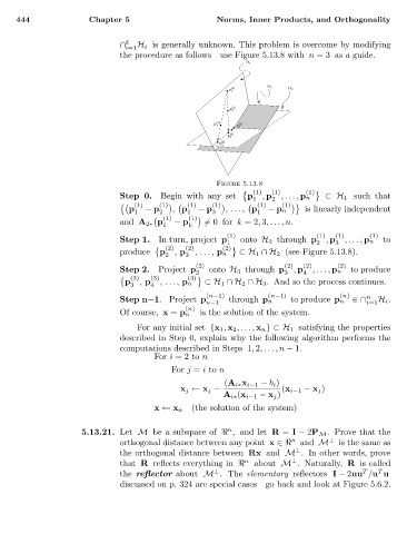
the procedure as follows—use Figure 5.13.8 with n =3 as a guide.

Figure 5.13.8
(1) (1) (1)
Step 0. Begin with any set p 1 , p 2 ,..., p n ⊂H 1 such that
(1) (1) (1) (1) (1) (1)
p − p , p − p ,. .., p is linearly independent
1 2 1 3 1 − p n
(1) (1)
and A 2∗ p − p =0 for k =2, 3,...,n.
1 k
(1) (1) (1) (1)
Step 1. In turn, project p 1 onto H 2 through p 2 , p 3 ,..., p n to
(2) (2) (2)
produce p 2 , p 3 ,. . . , p n ⊂H 1 ∩H 2 (see Figure 5.13.8).
(2) (2) (2) (2)
Step 2. Project p onto H 3 through p , p ,..., p n to produce
2 3 4
(3) (3) (3)
p , p ,. . . , p n ⊂H 1 ∩H 2 ∩H 3 . And so the process continues.
3 4
(n−1) (n−1) (n) n
Step n−1. Project p through p n to produce p n ∈∩ H i .
n−1 i=1
(n)
Of course, x = p n is the solution of the system.
Forany initial set {x 1 , x 2 ,..., x n }⊂H 1 satisfying the properties
described in Step 0, explain why the following algorithm performs the
computations described in Steps 1, 2,...,n − 1.
For i =2 to n
For j = i to n
(A i∗ x i−1 − b i )
x j ← x j − (x i−1 − x j )
A i∗ (x i−1 − x j )
(the solution of the system)
x ← x n
n
5.13.21. Let M bea subspace of , and let R = I − 2P M . Prove that the
n ⊥
orthogonal distance between any point x ∈ and M is the same as
⊥
the orthogonal distance between Rx and M . In other words, prove
n ⊥
that R reflects everything in about M . Naturally, R is called
T
T
the reflector about M . The elementary reflectors I − 2uu /u u
⊥
discussed on p. 324 are special cases—go back and look at Figure 5.6.2.