Page 65 - Matrix Analysis & Applied Linear Algebra

58 Chapter 2 Rectangular Systems and Echelon Forms

Since there are four unknowns but only two equations in this reduced system,
it is impossible to extract a unique solution for each unknown. The best we can
do is to pick two “basic” unknowns—which will be called the basic variables
and solve for these in terms of the other two unknowns—whose values must
remain arbitrary or “free,” and consequently they will be referred to as the free
variables. Although there are several possibilities for selecting a set of basic
variables, the convention is to always solve for the unknowns corresponding to
the pivotal positions—or, equivalently, the unknowns corresponding to the basic
columns. In this example, the pivots (as well as the basic columns) lie in the first
and third positions, so the strategy is to apply back substitution to solve the
reduced system (2.4.2) for the basic variables x 1 and x 3 in terms of the free
variables x 2 and x 4 . The second equation in (2.4.2) yields

x 3 = −x 4
and substitution back into the first equation produces
x 1 = −2x 2 − 2x 3 − 3x 4 ,
= −2x 2 − 2(−x 4 ) − 3x 4 ,
= −2x 2 − x 4 .

Therefore, all solutions of the original homogeneous system can be described by
saying
x 1 = −2x 2 − x 4 ,
x 2 is “free,”
(2.4.3)
x 3 = −x 4 ,
x 4 is “free.”
As the free variables x 2 and x 4 range over all possible values, the above ex-
pressions describe all possible solutions. For example, when x 2 and x 4 assume
the values x 2 = 1 and x 4 = −2, then the particular solution

x 1 =0,x 2 =1,x 3 =2,x 4 = −2
√
is produced. When x 2 = π and x 4 = 2, then another particular solution
√ √ √
x 1 = −2π − 2,x 2 = π, x 3 = − 2,x 4 = 2
is generated.
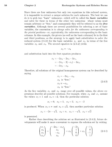
Rather than describing the solution set as illustrated in (2.4.3), future de-
velopments will make it more convenient to express the solution set by writing

       
x 1 −2x 2 − x 4 −2 −1
x 2
(2.4.4)
 x 2     1   0 
  =   = x 2   + x 4  
x 3 −x 4 0 −1
x 4 x 4 0 1