Page 66 - Matrix Analysis & Applied Linear Algebra

2.4 Homogeneous Systems 59

with the understanding that x 2 and x 4 are free variables that can range over
all possible numbers. This representation will be called the general solution
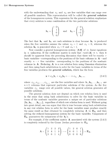
of the homogeneous system. This expression for the general solution emphasizes
that every solution is some combination of the two particular solutions

−2 −1
   
and  .
 1   0 
0 −1
h 1 =   h 2 = 
0 1
The fact that h 1 and h 2 are each solutions is clear because h 1 is produced
when the free variables assume the values x 2 = 1 and x 4 =0, whereas the
solution h 2 is generated when x 2 = 0 and x 4 =1.
Now consider a general homogeneous system [A|0]of m linear equations
in n unknowns. If the coefficient matrix is such that rank (A)= r, then it
should be apparent from the preceding discussion that there will be exactly r
basic variables—corresponding to the positions of the basic columns in A —and
exactly n − r free variables—corresponding to the positions of the nonbasic
columns in A . Reducing A to a row echelon form using Gaussian elimination
and then using back substitution to solve for the basic variables in terms of the
free variables produces the general solution, which has the form

h n−r , (2.4.5)
x = x f 1 h 1 + x f 2 h 2 + ··· + x f n−r
are the free variables and where h 1 , h 2 ,..., h n−r are
where x f 1 ,x f 2 ,...,x f n−r
n × 1 columns that represent particular solutions of the system. As the free
range over all possible values, the general solution generates all
variables x f i
possible solutions.
The general solution does not depend on which row echelon form is used
in the sense that using back substitution to solve for the basic variables in
terms of the nonbasic variables generates a unique set of particular solutions
{h 1 , h 2 ,..., h n−r }, regardless of which row echelon form is used. Without going
into great detail, one can argue that this is true because using back substitution
in any row echelon form to solve for the basic variables must produce exactly
the same result as that obtained by completely reducing A to E A and then
solving the reduced homogeneous system for the basic variables. Uniqueness of
E A guarantees the uniqueness of the h i ’s.
For example, if the coefficient matrix A associated with the system (2.4.1)
is completely reduced by the Gauss–Jordan procedure to E A

   
1223 1201
A =  2413  −→  0011  = E A ,
3614 0000