Page 232 - Mechanical Engineers' Handbook (Volume 2)

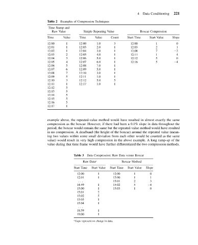
4 Data Conditioning 221

Table 2 Examples of Compression Techniques
Time Stamp and
Raw Value Simple Repeating Value Boxcar Compression
Time Value Time Value Count Start Time Start Value Slope
12:00 1 12:00 1.0 3 12:00 1 0
12:01 1 12:03 2.0 1 12:03 2 1
12:02 1 12:04 3.0 1 12:08 7 2
12:03 2 12:05 4.0 1 12:11 1 4
12:04 3 12:06 5.0 1 12:12 5 0
12:05 4 12:07 6.0 1 12:16 5 4
12:06 5 12:08 7.0 1
12:07 6 12:09 5.0 1
12:08 7 12:10 3.0 1
12:09 5 12:11 1.0 1
12:10 3 12:12 5.0 5
12:11 1 12:17 1.0 1
12:12 5
12:13 5
12:14 5
12:15 5
12:16 5
12:17 1

example above, the repeated-value method would have resulted in almost exactly the same
compression as the boxcar. However, if there had been a 0.1% slope in data throughout the
period, the boxcar would remain the same but the repeated-value method would have resulted
in no compression. A deadband (the height of the boxcar) around the repeated value (mean-
ing two values within some small deviation from each other would be counted as the same
value) would result in very high compression in the above example. A long ramp-up of the
value during that time frame would have further differentiated the two compression methods.

Table 3 Data Compression: Raw Data versus Boxcar
Raw Data a Boxcar Method

Start Time Start Value Start Time Start Value Slope
12:00 1 12:00 1 0
12:01 1 15:00 1 1
.. . 15:01 2 3
14:59 1 15:02 5 4
15:00 1 15:03 1 0
15:01 2
15:02 5
15:03 1
15:04 1
.. .
18:59 1
19:00 1

a
Gaps represent no change in data.