Page 228 - Mechanical Engineers' Handbook (Volume 2)

4 Data Conditioning 217

30

25

20
°C 15

10

5

0
-10 -5 0 5 10
Voltage, V

Legend

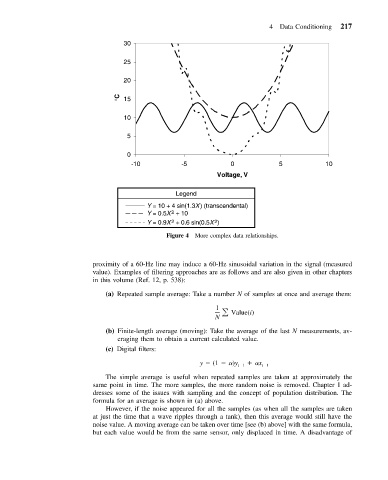
Y = 10 + 4 sin(1.3X) (transcendental)
2
Y = 0.5X + 10
Y = 0.9X + 0.6 sin(0.5X )
2
2
Figure 4 More complex data relationships.

proximity of a 60-Hz line may induce a 60-Hz sinusoidal variation in the signal (measured
value). Examples of filtering approaches are as follows and are also given in other chapters
in this volume (Ref. 12, p. 538):
(a) Repeated sample average: Take a number N of samples at once and average them:

1 Value(i)
N

(b) Finite-length average (moving): Take the average of the last N measurements, av-
eraging them to obtain a current calculated value.
(c) Digital filters:
y (1 )y i 1 x i 1

The simple average is useful when repeated samples are taken at approximately the
same point in time. The more samples, the more random noise is removed. Chapter 1 ad-
dresses some of the issues with sampling and the concept of population distribution. The
formula for an average is shown in (a) above.
However, if the noise appeared for all the samples (as when all the samples are taken
at just the time that a wave ripples through a tank), then this average would still have the
noise value. A moving average can be taken over time [see (b) above] with the same formula,
but each value would be from the same sensor, only displaced in time. A disadvantage of