Page 27 - Mechanical Engineers' Handbook (Volume 2)

16 Instrument Statics

x [56, 58, 60, 70, 72, 75, 77, 77, 82, 87, 92, 104, 125]
y [51, 60, 60, 52, 70, 65, 49, 60, 63, 61, 64, 84, 75]
At 0.05, the value of r is 0.55. Thus P[r calc 0.55] 0.05. The least-squares regression
equation is calculated to be y 39.32 0.30x, and the correlation coefficient is calculated
as r calc 0.61. Therefore, a satisfactory fit of the regression line to that data is inferred at
the 5% significance level (95% confidence level).

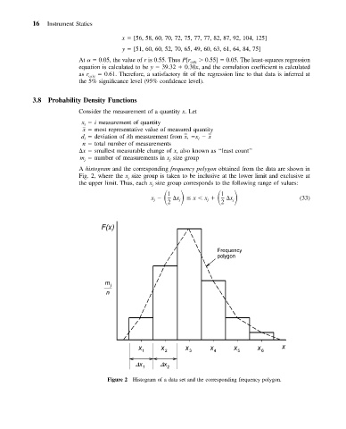
3.8 Probability Density Functions
Consider the measurement of a quantity x. Let
x i measurement of quantity
i
x most representative value of measured quantity
d deviation of ith measurement from , x x i x
i
n total number of measurements

x smallest measurable change of x, also known as ‘‘least count’’
m number of measurements in x size group
j
j
A histogram and the corresponding frequency polygon obtained from the data are shown in
Fig. 2, where the x size group is taken to be inclusive at the lower limit and exclusive at
j
the upper limit. Thus, each x size group corresponds to the following range of values:
j
x x x
1
1
j
2
x j j 2
x j (33)

Figure 2 Histogram of a data set and the corresponding frequency polygon.