Page 351 - Mechanical Engineers' Handbook (Volume 2)

342 Mathematical Models of Dynamic Physical Systems

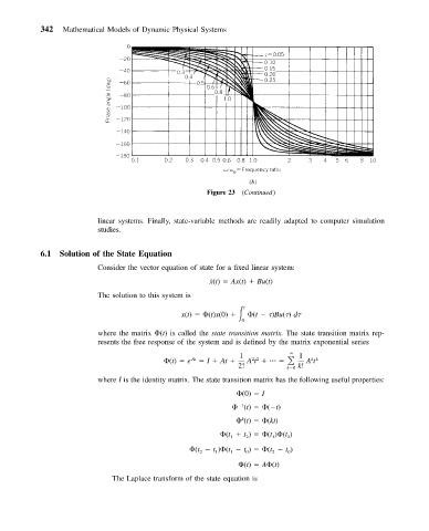
Figure 23 (Continued)

linear systems. Finally, state-variable methods are readily adapted to computer simulation
studies.

6.1 Solution of the State Equation

Consider the vector equation of state for a fixed linear system:
˙ x(t) Ax(t) Bu(t)
The solution to this system is
t
x(t) (t)x(0) (t )Bu( ) d
0
where the matrix (t) is called the state transition matrix. The state transition matrix rep-
resents the free response of the system and is defined by the matrix exponential series

1 At 1
kk
(t) e At I At 22 At
2! k 0 k!
where I is the identity matrix. The state transition matrix has the following useful properties:
(0) I
1
(t) ( t)
k
(t) (kt)
(t t ) (t ) (t )
2
1
2
1
(t t ) (t t ) (t t )
2
2
0
1
0
1
(t) A (t)
The Laplace transform of the state equation is