Page 389 - Mechanical Engineers' Handbook (Volume 2)

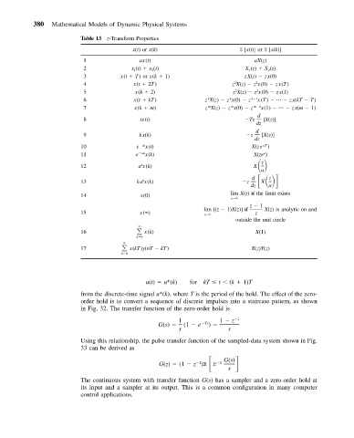
380 Mathematical Models of Dynamic Physical Systems

Table 13 z-Transform Properties
x(t)or x(k) Z Z [x(t)] or Z [x(k)]
Z
1 ax(t) aX(z)
2 x 1 (t) x 2 (t) X 1 (z) X 2 (z)
3 x(t T)or x(k 1) zX(z) zx(0)
2
2
4 x(t 2T) z X(z) z x(0) zx(T)
2
2
5 x(k 2) z X(z) z x(0) zx(1)
k
k
6 x(t kT) z X(z) z x(0) z k 1 x(T) zx(kT T)
m
m
7 x(k m) z X(z) z x(0) z m 1 x(1) zx(m 1)
d
8 tx(t) Tz [X(z)]
dz
d
9 kx(k) z [X(z)]
dz
aT
10 e at x(t) X(ze )
a
11 e ak x(k) X(ze )
z
k
12 a x(k) X
a
z
z
d
k
13 ka x(k) X
dz a
14 x(0) lim X(z) if the limit exists
z→
z 1
lim [(z 1)X(z)] if X(z) is analytic on and
15 x( ) z→1 z
outside the unit circle

16 x(k) X(1)
k 0

n
17 x(kT)y(nT kT) X(z)Y(z)
k 0
u(t) u*(k) for kT t (k 1)T
from the discrete-time signal u*(k), where T is the period of the hold. The effect of the zero-
order hold is to convert a sequence of discrete impulses into a staircase pattern, as shown
in Fig. 32. The transfer function of the zero-order hold is
1 1 z 1
G(s) (1 e Ts )
s s
Using this relationship, the pulse transfer function of the sampled-data system shown in Fig.
33 can be derived as
G(z) (1 z )ZZ
1 G(s)
1
L L L
s
The continuous system with transfer function G(s) has a sampler and a zero-order hold at
its input and a sampler at its output. This is a common configuration in many computer
control applications.