Page 483 - Mechanical Engineers' Handbook (Volume 2)

474 Closed-Loop Control System Analysis

M e
/
1 2 (75)
p
Peak Time t p
This is the time at which the peak occurs. It can be readily shown that

t (76)
p
d
It is important to note that given a set of time-domain design specifications, they can be
converted to an equivalent location of complex-conjugate poles. Figure 25 shows the allow-
able regions for complex-conjugate poles for different time-domain specifications.
For design purposes the following synthesis forms are useful:

1.8
(77a)
n
t r
0.6(1 M ) for 0 0.6 (77b)
p
4.6
(77c)
t s

5.6 Effects of an Additional Zero and an Additional Pole 2

If the standard second-order transfer function is modified due to a zero as
(s/ 1) 2
G (s) n n (78)
1
s 2 2 n
2
n
or due to an additional pole as
2
G (s) n (79)
2 2 2
(s/ 1)(s 2 s )
n
n
n
it is important to know how close the resulting step input response is to the standard second-
order step response. Following are several features of these additions:

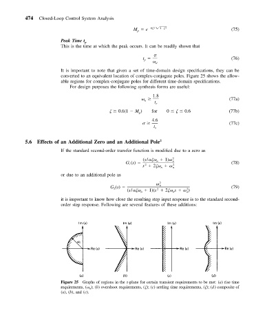
Figure 25 Graphs of regions in the s-plane for certain transient requirements to be met: (a) rise time
requirements, ( n ); (b) overshoot requirements, ( ); (c) settling time requirements, ( ); (d) composite of
(a), (b), and (c).