Page 478 - Mechanical Engineers' Handbook (Volume 2)

5 Closed-Loop Representation 469

or alternatively a transfer function called the closed-loop transfer function between the ref-
erence input and the output is defined:
Y(s) GG p
c
G (s) (58)
cl
R(s) 1 GG H
p
c
5.2 Open-Loop Transfer Function
The product of transfer functions within the loop, namely G G H, is referred to as the open-
c
p
loop transfer function or simply the loop transfer function:
G GG H (59)
ol
p
c
5.3 Characteristic Equation
The overall system dynamics given by Eq. (57) is primarily governed by the poles of the
closed-loop system or the roots of the closed-loop characteristic equation (CLCE):
1 GG H 0 (60)
c
p
It is important to note that the CLCE is simply
1 G 0 (61)
ol
This latter form is the basis of root-locus and frequency-domain design techniques dis-
cussed in Chapter 7.
The roots of the characteristic equation are referred to as poles. Specifically, the roots
of the open-loop characteristic equation (OLCE) are referred to as open-loop poles and those
of the closed loop are called closed-loop poles.

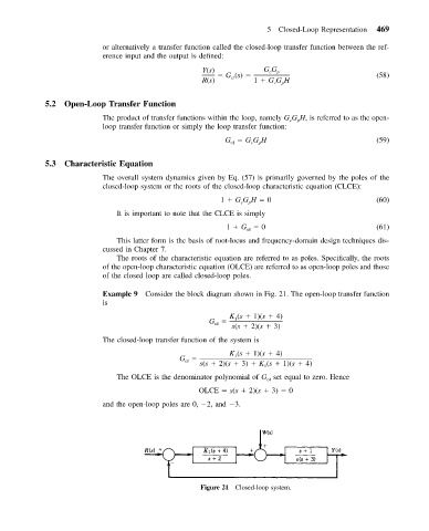
Example 9 Consider the block diagram shown in Fig. 21. The open-loop transfer function
is
K (s 1)(s 4)
G 1
ol
s(s 2)(s 3)
The closed-loop transfer function of the system is
K (s 1)(s 4)
G 1
cl
s(s 2)(s 3) K (s 1)(s 4)
1
The OLCE is the denominator polynomial of G set equal to zero. Hence
ol
OLCE s(s 2)(s 3) 0
and the open-loop poles are 0, 2, and 3.

Figure 21 Closed-loop system.