Page 547 - Mechanical Engineers' Handbook (Volume 2)

538 Control System Performance Modification

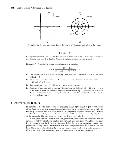
Figure 32 (a) Constant attenuation lines in the s-plane; (b) the corresponding loci in the z-plane.

1 G(z) 0

Exactly the same rules as used for the continuous-time case in the s-plane can be used for
the discrete case too. (See Section 5 for root-loci construction in the s-plane.)

Example 7 Consider the closed-loop characteristic equation
(z 1)(z 0.5)
1 K 0
(z 1)(z 0.9)(z 0.6)
R1: The system has n 3 poles indicating three branches. They start at 1, 0.9, and 0.6
with K 0.
R2: There are two finite zeros (m 2). Hence two of the branches terminate on the zeros
0.9 and 0.5 at K .
R3: One branch (n m 1) will go to along an asymptote.
R4: Sections of the root loci on the real line are between 0.9 and 1.0, 1.0 and , and
0.6 and 0.5; with this information the sketch shown in Fig. 33 can be easily obtained.
If additional features are needed, the rest of the root-loci construction rules can be
applied without change.

7 CONTROLLER DESIGN
In Sections 1–6 some useful tools for designing single-input–single-output systems were
given. Once the open-loop system is described, either by its set of poles and zeros or by its
frequency response, the root-locus method or frequency response method will indicate
whether the feedback system can be given an acceptable transient response by adjustment
of the loop gain. The steady-state accuracy can then be determined.
Often good transient performance and good steady-state performance cannot both be
achieved simply by adjusting a single parameter such as a loop gain. When this is the case,
it is necessary to modify the system dynamics. Either the dynamic properties of some com-
ponents in the loop need to be altered or additional components need to be inserted into the
loop. The process of modifying the system dynamics so as to allow the performance spec-
ifications to be met by subsequent loop gain adjustment is known as compensation.