Page 677 - Mechanical Engineers' Handbook (Volume 2)

668 Controller Design

continuous stable limit cycles with an amplitude corresponding to the resolution increment
(least significant bit in a digital system). In a high-resolution system, the magnitude of this
limit cycle may be so small that it is not noticeable. Similarly, Coulomb friction (Fig. 41e)
exhibits infinite gain around zero and a saturating behavior as amplitude increases. In this
case, however, the nonlinearity is usually a feedback loop around a mechanical load. When
the load is primarily inertial and has no backlash, friction may actually improve system
stability rather than decrease it. Of course, friction will also decrease system accuracy.

7.2 Complex Nonlinearities

As nonlinear elements become more complex, linear analysis becomes more complicated
and less realistic. However, linear techniques may still be of some use in estimating system
stability. For example, a servoactuator’s output velocity may be a nonlinear function of output
force as well as input drive current. For the example of Fig. 41d, system stability can be
explored by using linearized characteristics at selected operating points:
X
˙
˙
X
X
˙
i i F F (39)
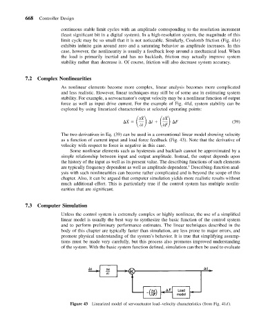
The two derivatives in Eq. (39) can be used in a conventional linear model showing velocity
as a function of current input and load force feedback (Fig. 43). Note that the derivative of
velocity with respect to force is negative in this case.
Some nonlinear elements such as hysteresis and backlash cannot be approximated by a
simple relationship between input and output amplitude. Instead, the output depends upon
the history of the input as well as its present value. The describing functions of such elements
1
are typically frequency dependent as well as amplitude dependent. Describing-function anal-
ysis with such nonlinearities can become rather complicated and is beyond the scope of this
chapter. Also, it can be argued that computer simulation yields more realistic results without
much additional effort. This is particularly true if the control system has multiple nonlin-
earities that are significant.

7.3 Computer Simulation
Unless the control system is extremely complex or highly nonlinear, the use of a simplified
linear model is usually the best way to synthesize the basic function of the control system
and to perform preliminary performance estimates. The linear techniques described in the
body of this chapter are typically faster than simulation, are less prone to major errors, and
promote physical understanding of the system’s behavior. It is true that simplifying assump-
tions must be made very carefully, but this process also promotes improved understanding
of the system. With the basic system function defined, simulation can then be used to evaluate

Figure 43 Linearized model of servoactuator load–velocity characteristics (from Fig. 41d).