Page 148 - Mechanical Engineers' Handbook (Volume 4)

9 Constructal Theory 137

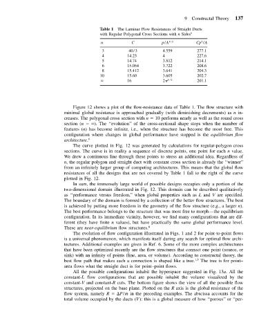
Table 1 The Laminar Flow Resistances of Straight Ducts
with Regular Polygonal Cross Sections with n Sides 6
2
n C p/A 1/2 Cp /A
3 40/3 4.559 277.1
4 14.23 4 227.6
5 14.74 3.812 214.1
6 15.054 3.722 208.6
8 15.412 3.641 204.3
10 15.60 3.605 202.7
16 2 1/2 201.1

Figure 12 shows a plot of the flow-resistance data of Table 1. The flow structure with
minimal global resistance is approached gradually (with diminishing decrements) as n in-
creases. The polygonal cross section with n 10 performs nearly as well as the round cross
section (n ). The ‘‘evolution’’ of the cross-sectional shape stops when the number of
features (n) has become infinite, i.e., when the structure has become the most free. This
configuration where changes in global performance have stopped is the equilibrium flow
architecture. 6
The curve plotted in Fig. 12 was generated by calculations for regular-polygon cross
sections. The curve is in reality a sequence of discrete points, one point for each n value.
We drew a continuous line through these points to stress an additional idea. Regardless of
n, the regular polygon and straight duct with constant cross section is already the ‘‘winner’’
from an infinitely larger group of competing architectures. This means that the global flow
resistances of all the designs that are not covered by Table 1 fall to the right of the curve
plotted in Fig. 12.
In sum, the immensely large world of possible designs occupies only a portion of the
two-dimensional domain illustrated in Fig. 12. This domain can be described qualitatively
as ‘‘performance versus freedom,’’ when global properties such as L and V are specified.
The boundary of the domain is formed by a collection of the better flow structures. The best
is achieved by putting more freedom in the geometry of the flow structure (e.g., a larger n).
The best performance belongs to the structure that was most free to morph—the equilibrium
configuration. In its immediate vicinity, however, we find many configurations that are dif-
ferent (they have finite n values), but have practically the same global performance level.
These are near-equilibrium flow structures. 6
The evolution of flow configuration illustrated in Figs. 1 and 2 for point-to-point flows
is a universal phenomenon, which manifests itself during any search for optimal flow archi-
tectures. Additional examples are given in Ref. 6. Some of the more complex architectures
that have been optimized recently are the flow structures that connect one point (source, or
sink) with an infinity of points (line, area, or volume). According to constructal theory, the
best flow path that makes such a connection is shaped like a tree. 1,5 The tree is for point–
area flows what the straight duct is for point–point flows.
All the possible configurations inhabit the hyperspace suggested in Fig. 13a. All the
constant-L flow configurations that are possible inhabit the volume visualized by the
constant-V and constant-R cuts. The bottom figure shows the view of all the possible flow
structures, projected on the base plane. Plotted on the R axis is the global resistance of the
flow system, namely R P/ ˙m in the preceding examples. The abscissa accounts for the
total volume occupied by the ducts (V): this is a global measure of how ‘‘porous’’ or ‘‘per-