Page 143 - Mechanical Engineers' Handbook (Volume 4)

132 Exergy Analysis, Entropy Generation Minimization, and Constructal Theory

of the power-producing compartment is too low, while when T T H,opt , too much of the
H
˙
unit heat input Q H bypasses the power compartment.
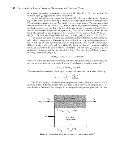
Another optimal hot-end temperature is revealed by the power plant model shown in
Fig. 9. The power plant is driven by a stream of hot single-phase fluid of inlet temperature
T and constant specific heat c . The model has two compartments. The one sandwiched
P
H
between the heat exchanger surface (T ) and the ambient (T ) operates reversibly. The other
L
HC
is a heat exchanger: for simplicity, the area of the T HC surface is assumed sufficiently large
that the stream outlet temperature is equal to T . The stream is discharged into the am-
HC
˙
bient. The optimal hot-end temperature for maximum W (or minimum S ˙ gen ) is 1,4 T HC,opt
˙
˙
(T T ) 1/2 . The corresponding first-law efficiency, W max /Q H ,is 1 (T /T ) 1/2 .
H
H L
L
The optimal allocation of a finite heat exchanger inventory between the hot end and the
cold end of a power plant is illustrated by the model with two heat exchangers proposed in
Ref. 3 and Fig. 10. The heat transfer rates are proportional to the respective temperature
˙
differences, Q ˙ H (UA) T and Q L (UA) T , where the thermal conductances (UA) H
L
L
H
H
˙
and (UA) account for the sizes of the heat exchangers. The heat input Q H is fixed (e.g., the
L
optimization is carried out for one unit of fuel burnt). The role of overall heat exchanger
inventory constraint is played by
(UA) (UA) UA (constant)
L
H
where UA is the total thermal conductance available. The power output is maximized, and
the entropy generation rate is minimized, when UA is allocated according to the rule
1
(UA) H,opt (UA) L,opt – UA
2
The corresponding maximum efficiency is, as expected, lower than the Carnot efficiency,
1 1 1
˙
4Q
T
H
L
T H T UA
H
The EGM modeling and optimization progress on power plants is extensive, and is
reviewed in Ref. 4. Similar models have also been used in the field of refrigeration, as we
saw already in Section 4. For example, in a steady-state refrigeration plant with two heat

Figure 9 Power plant driven by a stream of hot single-phase fluid. 1,4