Page 16 - Mechanics of Asphalt Microstructure and Micromechanics

Introduction and Fundamentals for Mathematics and Continuum Mechanics 9

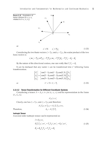
FIGURE 1.2 Illustration of x 3
frame rotation (0 x 1 x 2 x 3
x 3
rotated to 0 x 1 x 2 x 3 ).
x 1

x 2

0
x 2

x 1
or
'
'
e = Te e = T e (1-22)
i ij j
Considering the two basis vectors e i = T ir e r and e j = T js e s , the scalar product of the two
basis vectors is:
e • e = T e • T e = TT e • e = TT δ = T T = δ = δ

i j ir r js s ir js r s ir js rs i ir jr ij ij
By the nature of the directional cosines, one can verify that T ir T jr = d ij .
It can be deduced that any vector v can be transformed into v following frame
transformation.
−
⎧v ′ ⎫ ⎧ cos( 11),cos( 1' − 2),cos((', ) ⎫⎧v ⎫
'
13
⎪ 1 ⎪ ⎪ ⎪⎪ 1 ⎪
⎨
2
⎨ v ′ ⎬ = cos( ' 2 − 1 ),cos( ' 2 − 2 ),cos( ', ) 3 ⎬⎨ v ⎬
2
2
⎪ ⎪ ⎪ 3'− ⎪⎪ ⎪
⎪
1
3 3)
⎩ 3 ′ v ⎭ ⎩ cos( ' 3 − 1),cos( 2),cos( ', ⎭ ⎩ v 3 ⎭
or v = Tv v i = T ij (1-23)
1.5.4.2 Tensor Transformation for Different Coordinate Systems
Considering a tensor A = A ij e i e j in (e 1 , e 2 , e 3 ) and its representation in the frame
(e 1 , e 2 , e 3 ).
A ij e i e j
Clearly, one has e i = T ir e r and e j = T js e s and therefore:
A ij T ir e i T js e s = A ij T ir T js e r e s
Therefore, A rs = A ij T ir T js (1-24)
Isotropic Tensor
A second order isotropic tensor can be represented as:
I = δ e e

ij i j
(1-25)

δ = δ TT = T T = δ
'
ij pq pi qj qi qj ij