Page 255 - Mechanics of Asphalt Microstructure and Micromechanics

F inite Element Method and Boundar y Element Method 247

⎡ N 00,,, N 00,, ... N 00,, ⎤
⎢ 1 2 r ⎥
⎢
N = 0, N 0 0, , , N 0 0, ... , N ,0 ⎥
r r
2
1
⎢ 00 N ,,, N ... ,, N ⎥
00
,,
00
⎣ 1 2 r ⎦
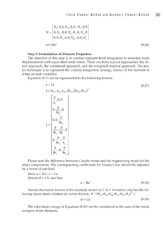
u = Nu q (8-26)

Step 3: Formulation of Element Properties
The objective of this step is to conduct element-level integration to associate node
displacements with equivalent node forces. There are three typical approaches: the di-
rect approach, the variational approach, and the weighted residual approach. The ma-
jor technique is to represent the volume integration (energy, forces) of the element in
terms of node variables.
Equation (8-1) can be represented in the following format:
ε = Lu (8-27)
ε = ( ε , ε , ε ,2 ε ,2 ε ,2 ε ) T
11 22 33 12 23 13
⎡ ∂ ⎤
⎢ ,, ⎥
00
⎢ x 1 ⎥
⎢ ∂ ⎥
⎢ 0, 0 , ⎥
⎢ x ∂ 2 ⎥
⎢ ∂ ⎥
⎢ 00 ,, ⎥
L = ⎢ ⎢ x ∂ 3 ⎥ ⎥ ⎥
⎢ ∂ ∂ ⎥
⎢ x ∂ , x ∂ 0 , ⎥
⎢ 2 1 ⎥
⎢ ∂ ∂ ∂ ⎥
⎢ 0, x ∂ , x ⎥
⎢ 3 2 ⎥
⎢ ∂ ∂ ⎥
⎢ ∂x 0 ,, ∂x ⎥
⎣ 3 1 ⎦
Please note the difference between Cauchy strain and the engineering strain for the
shear components. The corresponding coefficients for Hooke’s law should be adjusted
by a factor of one-half.
q
Since u = Nu , e = Lu.
Denote B = LN, one has:
ε = Bu q (8-28)
Denote the matrix format of the elasticity tensor as C (6 6 matrix); one has the fol-
T
lowing stress-strain relation (in vector format, σ = ( σ , σ , σ , σ , σ , σ ) ):
33
12
23
22
13
11
σ = C ε (8-29)
The total strain energy in Equation (8-23) can be considered as the sum of the strain
energies of the elements.