Page 257 - Mechanics of Asphalt Microstructure and Micromechanics

F inite Element Method and Boundar y Element Method 249

Step 6: Solution of the System Equation
The system equation may be linear or non-linear. There are various solution tech-
niques to solve the equation efficiently. The books on FEM listed in Section 8.1 have
excellent discussions on this topic.
Step 7: Check of Convergence Criteria
There are usually two types of convergence criterion — the displacement and the
force convergence criteria. Most of the commercial FEM codes provide guides on selec-
tion of these criteria.

8.2.2 Example
The following will use an example to consistently illustrate the seven steps mapped into
the formulations. The example is a 2D case, a beam of cantilever of w h l = 0.1 0.2 1
meter subjected a concentrated load of 1N (Figure 8.1). The material is isotropic and
8
linear elastic with E = 10 Pa and v = 0.25. 2D elements are used to model it. The follow-
ing only illustrates the problem setup process. It is suggested that readers accomplish
the solution with the help of Matlab and compare it with the solution using ABAQUS
or other commercial software.

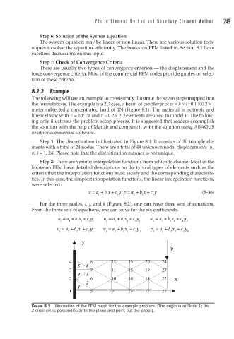
Step 1: The discretization is illustrated in Figure 8.1. It consists of 30 triangle ele-
ments with a total of 24 nodes. There are a total of 48 unknown nodal displacements (u i ,
v i , i = 1, 24) Please note that the discretization manner is not unique.
Step 2: There are various interpolation functions from which to choose. Most of the
books on FEM have detailed descriptions on the typical types of elements such as the
criteria that the interpolation functions must satisfy and the corresponding characteris-
tics. In this case, the simplest interpolation functions, the linear interpolation functions,
were selected.
u = a + b x c y v = a + b x c y (8-36)
+
+
,
1 1 1 2 2 2
For the three nodes, i, j, and k (Figure 8.2), one can have three sets of equations.
From the three sets of equations, one can solve for the six coefficients.
u = a + bx + c y u = a + bx + c y u = a + bx + y y
c
i 1 1 i 1 i j 1 1 j 1 j k 1 1 k 1 k
v = a + bx + c y v = a + bx + c y v = a + bx + c y
y
i 2 2 i 2 i j 2 2 j 2 j k 2 2 k 2 k
y
P

4 8 12 16 20 24
5 6
3 7 11 15 19 23
4 3
2 6 10 14 18 22 x
2
1
1 5 9 13 17 21

FIGURE 8.1 Illustration of the FEM mesh for the example problem. (The origin is at Node 1; the
Z direction is perpendicular to the plane and point out the paper).