Page 277 - Mechanics of Asphalt Microstructure and Micromechanics

F inite Element Method and Boundar y Element Method 269

−
'
H () (α = 1 − ) β H
(8-87)
−
K()α = σ + β Hα
y (8-88)
where q = the back stress or kinematic hardening center
p
e = plastic strain
a = the equivalent plastic strain for isotropic hardening
s = Cauchy stress tensor
• p •
•
q e a = the corresponding rate
–
s y , H, b = material constants
The constitutive model is a unified viscoplasticity model (Krempl, 1987). It might
not be applicable to pressure-sensitive materials such as granular material and bonded
granular materials. The Drucker-Prager (Drucker et al., 1952) yield function might be
better suited for this material. However, the discussion of the suitability and improve-
ment on the constitutive model are beyond the purpose of this section whose main fo-
cus is to illustrate the semi-implicit method. Implicit implementation of the Drucker-
Prager type of model using implicit method can be found in Wang et al. (2004). As this
constitutive model is one of the most advanced available constitutive models with de-
tailed material characterization, its implementation constitutes a good example. The
SHRP constitutive model is a very complicated model, mathematically, and the set of
equations has the following features:
• High nonlinearity
• Rate dependency
• Numerical stiffness
The implementation of this constitutive model is quite representative of the imple-
mentation of other viscoplasticity and elastoplasticity models. An analysis of the phys-
ical structure of the model is helpful. For example, the elastoplasticity model with linear
elasticity could be deduced from the general model by setting C = 0, i = −3 9 [see Equa-
i
tion (8-69) above] and canceling out the viscous component.
8.6.3 Finite Incremental Constitutive Equations
Elastoplasticity Component
Equation 8-64 is a generalized differential equation. The actual equations of evolution
in this case were Equations (8-81), (8-82), and (8-83). The several variables requiring
updates are stresses, kinematic and isotropic hardening variables, plastic strains, etc.
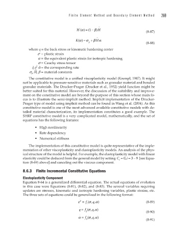
The three sets of equations could be generalized in the following format:
.
ε = f (, α) (8-89)
p
σ q,
1
.
q = f (,σ q, )α
2 (8-90)
.
α = f σ (, , α)
q
3 (8-91)