Page 87 - Mechanics of Asphalt Microstructure and Micromechanics

80 Ch a p t e r Th r e e

from its lower adjacent section (b), and the closest point from its upper adjacent section
(d) are selected as the surrounding points. These four points and the contact point can
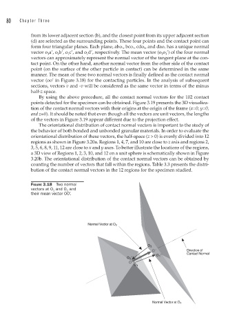
form four triangular planes. Each plane, abo 1 , bco 1 , cdo 1 , and dao 1 has a unique normal
vector o 1 a’, o 1 b’, o 1 c’, and o 1 d’, respectively. The mean vector (o 1 o 1 ’) of the four normal
vectors can approximately represent the normal vector of the tangent plane at the con-
tact point. On the other hand, another normal vector from the other side of the contact
point (on the surface of the other particle in contact) can be determined in the same
manner. The mean of these two normal vectors is finally defined as the contact normal
vector (oo’ in Figure 3.18) for the contacting particles. In the analysis of subsequent
sections, vectors v and -v will be considered as the same vector in terms of the minus
half-z space.
By using the above procedure, all the contact normal vectors for the 102 contact
points detected for the specimen can be obtained. Figure 3.19 presents the 3D visualiza-
tion of the contact normal vectors with their origins at the origin of the frame (x=0, y=0,
and z=0). It should be noted that even though all the vectors are unit vectors, the lengths
of the vectors in Figure 3.19 appear different due to the projection effect.
The orientational distribution of contact normal vectors is important to the study of
the behavior of both bonded and unbonded granular materials. In order to evaluate the
orientational distribution of these vectors, the half-space (z > 0) is evenly divided into 12
regions as shown in Figure 3.20a. Regions 1, 4, 7, and 10 are close to z axis and regions 2,
3, 5, 6, 8, 9, 11, 12 are close to x and y axes. To better illustrate the locations of the regions,
a 3D view of Regions 1, 2, 3, 10, and 12 on a unit sphere is schematically shown in Figure
3.20b. The orientational distribution of the contact normal vectors can be obtained by
counting the number of vectors that fall within the regions. Table 3.3 presents the distri-
bution of the contact normal vectors in the 12 regions for the specimen studied.

FIGURE 3.18 Two normal
vectors at O 1 and O 2 and
their mean vector OO’.