Page 55 - Mechatronic Systems Modelling and Simulation with HDLs

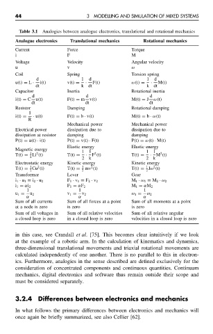
44 3 MODELLING AND SIMULATION OF MIXED SYSTEMS

Table 3.1 Analogies between analogue electronics, translational and rotational mechanics
Analogue electronics Translational mechanics Rotational mechanics
Current Force Torque
i F M
Voltage Velocity Angular velocity
u v ω
Coil Spring Torsion spring
d 1 d 1 d
u(t) = L · i(t) v(t) = · F(t) ω(t) = · M(t)
dt k dt k dt
Capacitor Inertia Rotational inertia
d d d
i(t) = C u(t) F(t) = m v(t) M(t) = J ω(t)
dt dt dt
Resistor Damping Rotational damping
1
i(t) = · u(t) F(t) = b · v(t) M(t) = b · ω(t)
R
Mechanical power Mechanical power
Electrical power dissipation due to dissipation due to
dissipation at resistor damping damping
P(t) = u(t) · i(t) P(t) = v(t) · F(t) P(t) = ω(t) · M(t)
Elastic energy Elastic energy
Magnetic energy 1 1 1 1
1
2
2
2
T(t) = Li (t) T(t) = · F (t) T(t) = · M (t)
2 2 k 2 k
Electrostatic energy Kinetic energy Kinetic energy
2
2
1
2
1
T(t) = Cu (t) T(t) = 1 mv (t) T(t) = Jω (t)
2 2 2
Transformer Lever Gear
i 1 · u 1 = i 2 · u 2 F 1 · v 1 = F 2 · v 2 M 1 · ω 1 = M 2 · ω 2
i 1 = αi 2 F 1 = αF 2 M 1 = αM 2
1 1 1
u 1 = u 2 v 1 = v 2 ω 1 = ω 2
α α α
Sum of all currents Sum of all forces at a point Sum of all moments at a point
at a node is zero is zero is zero
Sum of all voltages in Sum of all relative velocities Sum of all relative angular
a closed loop is zero in a closed loop is zero velocities in a closed loop is zero
in this case, see Crandall et al. [75]. This becomes clear intuitively if we look
at the example of a robotic arm. In the calculation of kinematics and dynamics,
three-dimensional translational movements and triaxial rotational movements are
calculated independently of one another. There is no parallel to this in electron-
ics. Furthermore, analogies in the sense described are defined exclusively for the
consideration of concentrated components and continuous quantities. Continuum
mechanics, digital electronics and software thus remain outside their scope and
must be considered separately.

3.2.4 Differences between electronics and mechanics

In what follows the primary differences between electronics and mechanics will
once again be briefly summarized, see also Cellier [62].