Page 449 - Mechatronics for Safety, Security and Dependability in a New Era

Ch87-I044963.fm Page 433 Monday, August 7, 2006 11:32 AM
11:32 AM
Monday, August 7,2006
Page 433
Ch87-I044963.fm
433
433
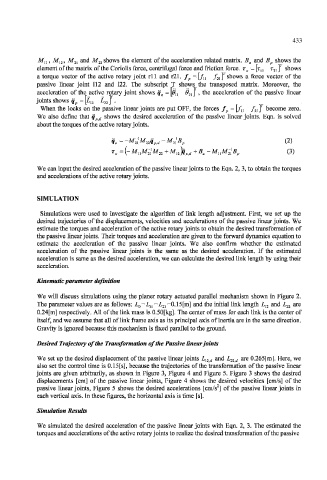
M u, M l2, M 2I and M 22 shows the element of the acceleration related matrix. B a and B p shows the
element of the matrix of the Coriolis force, centrifugal force and friction force. r o = [r n r 21 ]' shows
a torque vector of the active rotary joint rll and r21. f =\f n f 21f shows a force vector of the
passive linear joint 112 and 122. The subscript T shows the transposed matrix. Moreover, the
acceleration of the active rotary joint shows q a =[0 U & 2l\ , the acceleration of the passive linear
joints shows q p = [L l2 L 22\ .
When the locks on the passive linear joints are put OFF, the forces f p =[f u f 2]]' become zero.
We also define that q p d shows the desired acceleration of the passive linear joints. Eqn. is solved
about the torques of the active rotary joints.

(2)
q a=-M;lM 21q PtJ-M;\B p
(3)
z a =(-M uM 2:M 22 +M n)i p4 +B a -M nM 2:B p
We can input the desired acceleration of the passive linear joints to the Eqn. 2, 3, to obtain the torques
and accelerations of the active rotary joints.

SIMULATION

Simulations were used to investigate the algorithm of link length adjustment. First, we set up the
desired trajectories of the displacements, velocities and accelerations of the passive linear joints. We
estimate the torques and acceleration of the active rotary joints to obtain the desired transformation of
the passive linear joints. Their torques and acceleration are given to the forward dynamics equation to
estimate the acceleration of the passive linear joints. We also confirm whether the estimated
acceleration of the passive linear joints is the same as the desired acceleration. If the estimated
acceleration is same as the desired acceleration, we can calculate the desired link length by using their
acceleration.

Kinematic parameter definition

We will discuss simulations using the planer rotary actuated parallel mechanism shown in Figure 2.
The parameter values are as follows: L 0 = L u = L 2] =0.15[m] and the initial link length L n and L 22 are
0.24[m] respectively. All of the link mass is 0.50[kg]. The center of mass for each link is the center of
itself, and we assume that all of link frame axis as its principal axis of inertia are in the same direction.
Gravity is ignored because this mechanism is fixed parallel to the ground.

Desired Trajectory of the Transformation of the Passive linear joints
We set up the desired displacement of the passive linear joints L 12d and L 22d are 0.265[m]. Here, we
also set the control time is 0.15[s], because the trajectories of the transformation of the passive linear
joints are given arbitrarily, as shown in Figure 3, Figure 4 and Figure 5. Figure 3 shows the desired
displacements [cm] of the passive linear joints, Figure 4 shows the desired velocities [cm/s] of the
2
passive linear joints, Figure 5 shows the desired accelerations [cm/s ] of the passive linear joints in
each vertical axis. In these figures, the horizontal axis is time [s].

Simulation Results
We simulated the desired acceleration of the passive linear joints with Eqn. 2, 3. The estimated the
torques and accelerations of the active rotary joints to realize the desired transformation of the passive