Page 540 - Modelling in Transport Phenomena A Conceptual Approach

520 APPENDIX A. MATWEMATXU P.WLIMINARIES

2
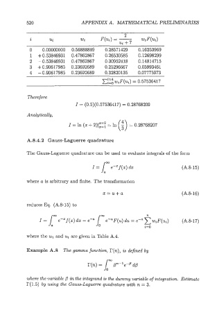
i ui Wi qui) = - wiF(ui)
ui + 7
0 0.00000000 0.56888889 0.28571429 0.16253969
1 + 0.53846931 0.47862867 0.26530585 0.12698299
2 - 0.53846931 0.47862867 0.30952418 0.14814715
3 + 0.90617985 0.23692689 0.25296667 0.05993461
4 - 0.90617985 0.23692689 0.32820135 0.07775973

Therefore
I = (0.5)(0.57536417) = 0.28768209

Analytically,
I = In (x -I- 2)1:1: = In

A.8.4.2 Gauss-Laguerre quadrature

The GaussLaguerre quadrature can be used to evaluate integrals of the form

(A.8-15)

where a is arbitrary and finite. The transformation

x=u+a (A.8-16)

reduces Eq. (A.8-15) to

n
I = I" e-"f(x) dx = e-a 1" e-"F(u) du = e-a wiF(u6) (A.8-17)
i=O
where the wi and ui are given in Table A.4.

Example A.8 The gamma function, r(n), is defined by

where the variable p in the integrand is the dummy variable of integration. Estimate
r(1.5) by using the Gauss-Laguem quadrature with n = 3.