
Page 538 - Modelling in Transport Phenomena A Conceptual Approach
P. 538
518 APPENDIX A. MATHEMATICAL PRELIM2NARIES
The value of the integral can be calculated from Eq. (A.8-9) as
0 = 100 I19.65 + 2(26.74 + 32.80 + 37.74 + 41.75 + 45.06 + 47.83) + 50.161
2
= 26,683 cal/ mol
Simpson’s rule with n = 4
From Eq. (A.8-12)
1000 - 300 = 175
AT =
4
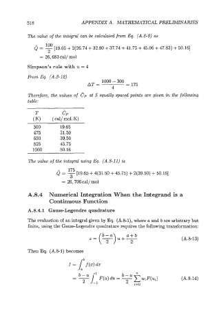
Therefore, the values of cp at 5 equally spaced points are given in the following
table:
T CP
( K) ( cal/ mol. K)
~
300 19.65
475 31.50
650 39.50
825 45.75
1000 50.16
The value of the integral using Eq. (A.8-11) aS
Q=-- 175 [19.65 + 4(31.50 + 45.75) + 2(39.50) + 50.161
3
= 26,706 cal/ mol
A.8.4 Numerical Integration When the Integrand is a
Continuous Function
A.8.4.1 Gauss-Legendre quadrature
The evaluation of an integral given by Eq. (A.&l), where a and b are arbitrary but
finite, using the Gauss-Legendre quadrature requires the following transformation:
x= (?>..- a+b
2 (A.8-13)
Then Eq. (A.8-1) becomes
(A.8-14)