Page 65 - Modelling in Transport Phenomena A Conceptual Approach

46 CHAPTER 3. INTERPHASE TRANSPORT

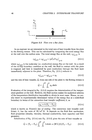
Figure 3.3 Flow over a flat plate.

As an engineer we are interested in the total rate of heat transfer from the plate
to the flowing stream. This can be calculated by integrating the total energy flux
at the wall over the surface area. The total energy flux at the wall, e,l,,o, is
(3.2-1)

where qvlY=o is the molecular (or, conductive) energy flux at the wall. As a result
of the no-slip boundary condition at the wall, the fluid in contact with the plate
is stagnant and heat is transferred by pure conduction through the fluid layer
immediately adjacent to the plate. Therefore, Eq. (3.2-1) reduces to

eYly=0 = QYIar=O = 4u (3.2-2)
and the rate of heat transfer, Q, from one side of the plate to the flowing stream is

Q = Jd" Jd" qw dxdz (3.2-3)

Evaluation of the integral in Eq. (3.2-3) requires the determination of the temper-
ature gradient at the wall. However, the fluid motion makes the analytical solution
of the temperature distribution impossible to obtain in most cases. Hence, we usu-
ally resort to experimentally determined values of the energy flux at a solid-fluid
boundary in terms of the convection heat transfer weficient, h, as
(3.2-4)

which is known as Newton's law of woling. The convection heat transfer coef-
ficient, h, has the units of W/m2.K. It depends on the fluid flow mechanism,
fluid properties (density, viscosity, thermal conductivity, heat capacity) and flow
geometry.
Substitution of Eq. (3.2-4) into Eq. (3.2-3) gives the rate of heat transfer as

Q = (T, - Tm) Jd" 1" hdxdz = (WL)(h)(T, - T,) (3.2-5)