Page 352 - Modern Analytical Chemistry

1400-CH09 9/9/99 2:13 PM Page 335

Chapter 9 Titrimetric Methods of Analysis 335

9 7
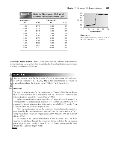
Table .1 Data for Titration of 50.0 mL of 1.8
0.100 M Fe 2+ with 0.100 M Ce 4+ 1.6
1.4
Volume Ce 4+ Volume Ce 4+ E 1.2
(mL) E (V) (mL) E (V) 1
0.8
5.00 0.711 55.00 1.64
0.6
10.00 0.731 60.00 1.66 0 20 40 60 80 100
15.00 0.745 65.00 1.67 Volume of Ce 4+
20.00 0.757 70.00 1.68
25.00 0.767 75.00 1.68 Figure 9.34
Redox titration curve for 50.0 mL of 0.100 M
30.00 0.777 80.00 1.69
Fe 2+ with 0.100 M Ce 4+ in 1 M HClO 4 .
35.00 0.789 85.00 1.69
40.00 0.803 90.00 1.69
45.00 0.823 95.00 1.70
50.00 1.23 100.00 1.70

Sketching a Redox Titration Curve As we have done for acid–base and complexo-
metric titrations, we now show how to quickly sketch a redox titration curve using a
minimum number of calculations.

9
EXAMPLE .11
Sketch a titration curve for the titration of 50.0 mL of 0.100 M Fe 2+ with 0.100
M Ce 4+ in a matrix of 1 M HClO 4 . This is the same titration for which we
previously calculated the titration curve (Table 9.17 and Figure 9.34).

SOLUTION
We begin by drawing axes for the titration curve (Figure 9.35a). Having shown
that the equivalence point volume is 50.0 mL, we draw a vertical line
intersecting the x-axis at this volume (Figure 9.35b).
Before the equivalence point, the solution’s electrochemical potential is
determined by the concentration of excess Fe 2+ and the concentration of Fe 3+
produced by the titration reaction. Using values from Table 9.17, we plot E for
5.0 mL and 45.0 mL of titrant (Figure 9.35c).
After the equivalence point, the solution’s electrochemical potential is
3+
determined by the concentration of excess Ce 4+ and the concentration of Ce .
Using values from Table 9.17, we plot points for 60.0 mL and 80.0 mL of titrant
(Figure 9.35d).
To complete an approximate sketch of the titration curve, we draw
separate straight lines through the two points before and after the equivalence
point (Figure 9.35e). Finally, a smooth curve is drawn to connect the three
straight-line segments (Figure 9.35f).