Page 367 - Modern Analytical Chemistry

1400-CH09 9/9/99 2:13 PM Page 350

350 Modern Analytical Chemistry

Thus, there is 2.43 mg of ascorbic acid in the 5.00-mL sample, or 48.6 mg/100
mL of orange juice.

9D.5 Evaluation of Redox Titrimetry
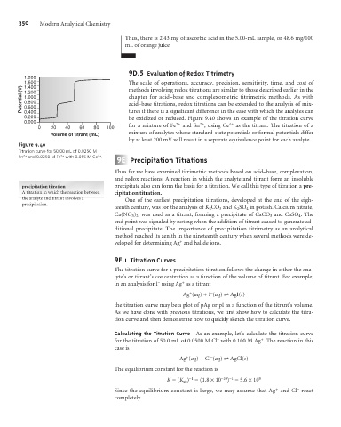
1.800
1.600 The scale of operations, accuracy, precision, sensitivity, time, and cost of
1.400
Potential (V) 1.200 chapter for acid–base and complexometric titrimetric methods. As with
methods involving redox titrations are similar to those described earlier in the
1.000
0.800
acid–base titrations, redox titrations can be extended to the analysis of mix-
0.600
0.400
0.200 tures if there is a significant difference in the ease with which the analytes can
be oxidized or reduced. Figure 9.40 shows an example of the titration curve
0.000 2+ 2+ 4+
0 20 40 60 80 100 for a mixture of Fe and Sn , using Ce as the titrant. The titration of a
mixture of analytes whose standard-state potentials or formal potentials differ
Volume of titrant (mL)
by at least 200 mV will result in a separate equivalence point for each analyte.
Figure 9.40
Titration curve for 50.00 mL of 0.0250 M
4+
Sn 2+ and 0.0250 M Fe 2+ with 0.055 M Ce . 9 E Precipitation Titrations
Thus far we have examined titrimetric methods based on acid–base, complexation,
and redox reactions. A reaction in which the analyte and titrant form an insoluble
precipitation titration precipitate also can form the basis for a titration. We call this type of titration a pre-
A titration in which the reaction between cipitation titration.
the analyte and titrant involves a One of the earliest precipitation titrations, developed at the end of the eigh-
precipitation.
teenth century, was for the analysis of K 2 CO 3 and K 2 SO 4 in potash. Calcium nitrate,
Ca(NO 3 ) 2 , was used as a titrant, forming a precipitate of CaCO 3 and CaSO 4 . The
end point was signaled by noting when the addition of titrant ceased to generate ad-
ditional precipitate. The importance of precipitation titrimetry as an analytical
method reached its zenith in the nineteenth century when several methods were de-
+
veloped for determining Ag and halide ions.
9 E.1 Titration Curves
The titration curve for a precipitation titration follows the change in either the ana-
lyte’s or titrant’s concentration as a function of the volume of titrant. For example,
+
–
in an analysis for I using Ag as a titrant
–
+
Ag (aq)+I (aq) t AgI(s)
the titration curve may be a plot of pAg or pI as a function of the titrant’s volume.
As we have done with previous titrations, we first show how to calculate the titra-
tion curve and then demonstrate how to quickly sketch the titration curve.

Calculating the Titration Curve As an example, let’s calculate the titration curve
–
+
for the titration of 50.0 mL of 0.0500 M Cl with 0.100 M Ag . The reaction in this
case is
+
–
Ag (aq)+Cl (aq) t AgCl(s)
The equilibrium constant for the reaction is
–1
) = 5.6 ´10
K =(K sp ) = (1.8 ´10 –10 –1 9
+
–
Since the equilibrium constant is large, we may assume that Ag and Cl react
completely.