Page 369 - Modern Analytical Chemistry

1400-CH09 9/9/99 2:13 PM Page 352

352 Modern Analytical Chemistry

9.00 9
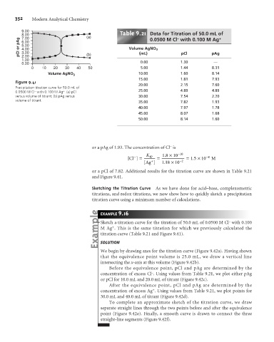
8.00 (a) Table .21 Data for Titration of 50.0 mL of
7.00
pCl or pAg 6.00 Volume AgNO 3
0.0500 M Cl with 0.100 M Ag
–
+
5.00
4.00
3.00
2.00
1.00 (b) (mL) pCl pAg
0.00 0.00 1.30 —
0 10 20 30 40 50 5.00 1.44 8.31
Volume AgNO 3 10.00 1.60 8.14
15.00 1.81 7.93
Figure 9.41
20.00 2.15 7.60
Precipitation titration curve for 50.0 mL of
–
+
0.0500 M Cl with 0.100 M Ag . (a) pCl 25.00 4.89 4.89
versus volume of titrant; (b) pAg versus 30.00 7.54 2.20
volume of titrant.
35.00 7.82 1.93
40.00 7.97 1.78
45.00 8.07 1.68
50.00 8.14 1.60

–
or a pAg of 1.93. The concentration of Cl is
K sp 18 - 10 - 8
. ´10
. ´ 10
[Cl - ] = = =15 M
[Ag + ] . 118 ´10 - 2

or a pCl of 7.82. Additional results for the titration curve are shown in Table 9.21
and Figure 9.41.
Sketching the Titration Curve As we have done for acid–base, complexometric
titrations, and redox titrations, we now show how to quickly sketch a precipitation
titration curve using a minimum number of calculations.

9
EXAMPLE .16
–
Sketch a titration curve for the titration of 50.0 mL of 0.0500 M Cl with 0.100
+
M Ag . This is the same titration for which we previously calculated the
titration curve (Table 9.21 and Figure 9.41).
SOLUTION

We begin by drawing axes for the titration curve (Figure 9.42a). Having shown
that the equivalence point volume is 25.0 mL, we draw a vertical line
intersecting the x-axis at this volume (Figure 9.42b).
Before the equivalence point, pCl and pAg are determined by the
–
concentration of excess Cl . Using values from Table 9.21, we plot either pAg
or pCl for 10.0 mL and 20.0 mL of titrant (Figure 9.42c).
After the equivalence point, pCl and pAg are determined by the
+
concentration of excess Ag . Using values from Table 9.21, we plot points for
30.0 mL and 40.0 mL of titrant (Figure 9.42d).
To complete an approximate sketch of the titration curve, we draw
separate straight lines through the two points before and after the equivalence
point (Figure 9.42e). Finally, a smooth curve is drawn to connect the three
straight-line segments (Figure 9.42f).