Page 218 - Modern Control Systems

Chapter 3 State Variable Models

1(1/5)
<f>2 2(s) = 1 2 2 (3.91)
1 + 3s" + 2.r .v + 3s + 2
Therefore, the state transition matrix in Laplace transformation form is

(s + 3)/(5 2 + 35 + 2) -2/(5 2 + 35 + 2)"
*(*) = 2 2 (3.92)
1/(5 + 35 + 2) s/(s + 35 + 2)
The factors of the characteristic equation are (5 + 1) and (s + 2), so that

(5 + 1)(5 + 2) = 5 2 + 35 + 2.
Then the state transition matrix is

2
21
(2e- { - e~ ') (-2e~ l + 2e~ )
¢(0 = X-'Ws)} = 2 (3.93)
(e *-* ) (-«?-' + 2eT ')
The evaluation of the time response of the RLC network to various initial condi-
tions and input signals can now be evaluated by using Equation (3.80). For example,
when *i(0) = x 2(0) = 1 and u{t) = 0, we have

2
*i(0 f V <~
= *(') = 2 (3.94)
_x 2(t)_ _1_ _e~ '_
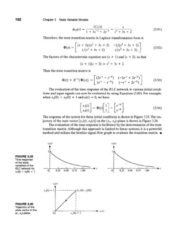
The response of the system for these initial conditions is shown in Figure 3.25. The tra-
jectory of the state vector [x x{t), x 2(t)] on the (jq, .v 2 )-pl ane is shown in Figure 3.26.
The evaluation of the time response is facilitated by the determination of the state
transition matrix. Although this approach is limited to linear systems, it is a powerful
method and utilizes the familiar signal-flow graph to evaluate the transition matrix. •

•h(t)

FIGURE 3.25
Time response
of the state
variables of the
RLC network for *>t
x 1(0)=x 2(0) = 1. 0.25 0.50 0.75 1.00

(JT,(0),.V 2 (0))

FIGURE 3.26
Trajectory of the
state vector in the * .v,(r)
, x 2)-plane. .V,(0) = 1