Page 22 - Modern Control Systems

XViii Preface

Select K a.
IVet-JU, *
t=[0:0.01:1];
nc=[Ka*5];dc=[1]; sysc=tf(nc,dc);
ng-[1];dg-[1 20 0]; sysg-tf(ng.dg);
Compute the
sys1=series(sysc,sysg); ]
closed-loop
sys=TeedbacK(sysi, pj); f *
y=step(sys,t); J transfer function.
plot(t,y), grid
xlabeI(Time (s)')
ylabelCy(ty)
(a)

1.2
K a = 60.
1

0.8
K a = 30.
§ 0.6
0.4

0.2

0
0 0.1 0.2 0.3 0.4 0.5 0.6 0.7 0.8 0.9 1
Time (s)
(b)

Learning Enhancement. Each chapter begins with a chapter preview describing
the topics the student can expect to encounter. The chapters conclude with an
end-of-chapter summary, skills check, as well as terms and concepts. These sec-
tions reinforce the important concepts introduced in the chapter and serve as a
reference for later use.
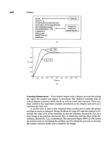
A second color is used to add emphasis when needed and to make the graphs
and figures easier to interpret. Design Problem 4.4, page 297, asks the student to de-
termine the value of K of the controller so that the response, denoted by Y(s), to a
step change in the position, denoted by R(s), is satisfactory and the effect of the dis-
turbance, denoted by T d(s)> is minimized.The associated Figure DP4.4, p. 298, assists
the student with (a) visualizing the problem and (b) taking the next step to develop
the transfer function model and to complete the design.