Page 190 - Modern Spatiotemporal Geostatistics

Modifications of BME Analysis 171

sought at the point p k (k ^ i). Equations 9.13-9.15 reduce to the following
system of equations

and

and the posterior pdf (given and

where, as usual, Equation 9.17 is the vectorial form of the
BME equation (Eq. 7.6, p. 137). Other posterior operators % (as described in
Chapters 6 and 7) could also be implemented. In fact, any possible combination
of hard and soft data for X(p) and Y(p) could be considered in a similar
fashion. This is a good point to pause and discuss a simple example.
EXAMPLE 9.3: Consider the points p i (i = 1, 2, 3, 4). The hard and soft data
available include, x hard = (xi, Xz), Xaoft = X3, and \data = (\hard, Xsoft)
for the primary field X(p); and i/> hard = (V>i, ^2), ^ soft = (fa, ^4) and
Tfidata = (V'hard. V"Soft) f°r the secondary field Y(p). An estimate of X(p
is sought at point p k, so that \ map = (Xdata, Xk)- Known statistics are the
means, variances, (centered) covariances, and cross-covariances between all
points considered. The g a functions (a = 0, 1,..., 44) are shown in Table
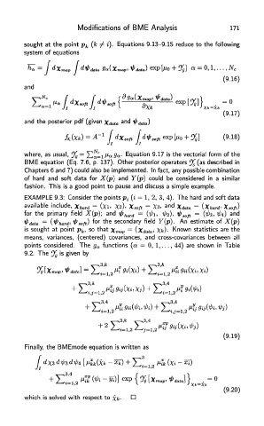
9.2. The y g is given by

Finally, the BMEmode equation is written as

which is solved with respect to