Page 191 - Modern Spatiotemporal Geostatistics

172 Modern Spatiotemporal Geostatistics — Chapter 9

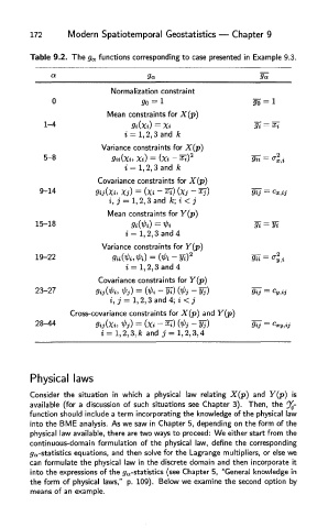
Table 9.2. The g a functions corresponding to case presented in Example 9.3.

Normalization constraint
0 3o = l
Mean constraints for X(p)
1 - 4 9i(Xi) = Xi

i = 1,2,3 and k

Variance constraints for X(p)
5-8 gu(xi, Xi) = (Xi ~ xtf

i = 1,2,3 and k

Covariance constraints for X(p)

9-14 9ij(Xi, Xj) = (Xi ~ x$(Xj - Xj )

i, j = 1,2, 3 and k; i < j

Mean constraints for Y(p)
15-18
i = 1,2,3 and 4
Variance constraints for Y(p)
19-22
i = 1,2,3 and 4
Covariance constraints for Y(p)
23-27
i,j = 1,2,3 and 4; i <j

Cross-covariance constraints for X(p) and Y(p)
28-44
i = 1,2,3, kand j = l,2,3,4

Physical laws

Consider the situation in which a physical law relating X(p) and Y(p) is
available (for a discussion of such situations see Chapter 3). Then, the 9£-
function should include a term incorporating the knowledge of the physical law
into the BME analysis. As we saw in Chapter 5, depending on the form of the
physical law available, there are two ways to proceed: We either start from the
continuous-domain formulation of the physical law, define the corresponding
^-statistics equations, and then solve for the Lagrange multipliers, or else we
can formulate the physical law in the discrete domain and then incorporate it
into the expressions of the (^.-statistics (see Chapter 5, "General knowledge in
the form of physical laws," p. 109). Below we examine the second option by
means of an example.