Page 195 - Modern Spatiotemporal Geostatistics

176 Modern Spatiotemporal Geostatistics — Chapter 9

Equations 9.27 through 9.29 permit the body of available knowledge to reach
out and seek relations beyond its present state.

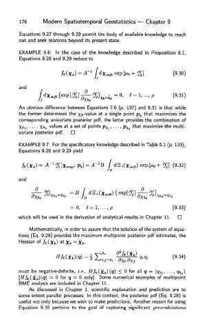
EXAMPLE 9.6: In the case of the knowledge described in Proposition 6.1,
Equations 9.28 and 9.29 reduce to

and

An obvious difference between Equations 7.6 (p. 137) and 9.31 is that while
the former determines the Xfc-value at a single point p k that maximizes the
corresponding univariate posterior pdf, the latter provides the combination of
Xki, • • • > Xk p values at a set of points p fcl, ..., p k that maximize the multi-
variate posterior pdf.

EXAMPLE 9.7: For the specificatory knowledge described in Table 6.1 (p. 133),
Equations 9.28 and 9.29 yield

and

which will be used in the derivation of analytical results in Chapter 11. D

Mathematically, in order to assure that the solution of the system of equa-
tions (Eq. 9.29) provides the maximum multipoint posterior pdf estimates, the
Hessian of

must be negative-definite, i.e., Hf K(Xk)(Q) < 0 for all q = (q kl, ..., Qk p)
[Hf K(x k)(Q) = 0 for q = 0 only]. Some numerical examples of multipoint
BME analysis are included in Chapter 11.
As discussed in Chapter 1, scientific explanation and prediction are to
some extent parallel processes. In this context, the posterior pdf (Eq. 9.28) is
useful not only because we wish to make predictions. Another reason for using
Equation 9.28 pertains to the goal of capturing significant generalizations