Page 197 - Neural Network Modeling and Identification of Dynamical Systems

188 5. SEMIEMPIRICAL NEURAL NETWORK MODELS OF CONTROLLED DYNAMICAL SYSTEMS

problems, we expect to have a continuous curve
of solutions.
We can see these considerations as an infor-
mal explanation of the ideas behind the homo-
topy continuation method [28,29] for the solu-
tion of nonlinear equation systems

F(w) = 0, (5.41)

where F: R n w → R n w is a smooth vector-valued
function. First, we choose a smooth vector-
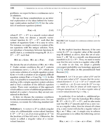
valued function G: R n w → R n w such that the FIGURE 5.10 Example of a continuous solution curve for
system of equations G(w) = 0 is easy to solve. H(τ,w) = 0.
For instance, we might construct a system of lin-
ear equations with the unique solution. Next,
we introduce a homotopy between functions G By the implicit function theorem, if the zero
vector 0 ∈ R n w is a regular value of the smooth
and F, that is, a continuous mapping H:[0,1]×
R n w → R n w such that map H defined as above, then the set of solu-
tions = H −1 (0) is a smooth one-dimensional
n w
H(0,w) = G(w), H(1,w) = F(w). (5.42) manifold in [0,1]× R . Thus, we need to make
sure that the zero vector is a regular value of H.
We denote the set of solutions of H(τ,w) = 0 by In order to do that, we adopt a globally
. Under certain conditions the set contains convergent probability-one homotopy approach
a continuous curve γ ⊂[0,1]× R , which con- [30,31], which relies on the parametrized Sard
n w
nects some solution of a simple equation system theorem [30].
G(w) = 0 with a solution of an original, difficult
q
equation system F(w) = 0 (see Fig. 5.10). In this Theorem 5. Let V be an open subset of R and let
m
case, it is possible to numerically trace this curve U be an open subset of R . Assume that the vector-
r
p
starting with a simple equation system solution valued function f: V × U → R is C -smooth with
p
and to find a solution of the difficult equation r> max{0,m − p}. If a zero vector 0 ∈ R is a reg-
system. There exist variations of this approach ular value of f, then for almost all (with respect to
which utilize a vector of additional parameters τ Lebesgue measure) a ∈ V it is also a regular value of
instead of a scalar τ; however, they are not con- a vector-valued function f a (·) = f(a,·).
sidered in this book.
At first, we discuss the existence conditions In particular, if we include n w additional pa-
for the abovementioned solution curve. For con- rameters a ∈ R n w into the homotopy H to obtain
n w
venience, we restate the following standard def- H: R n w ×[0,1]× R n w → R , and we also make
2
inition. sure that H is C -smooth and it has a zero vec-
tor as a regular value, then for almost all values
n
Definition 1. Avector v ∈ R is called a regular of a, a zero vector will also be a regular value of
value of a differentiable vector-valued function H a (τ,w) H(a,τ,w). A simple way to achieve
n
m
f: R → R (n m), if at every point u ∈ f −1 (v) this guarantee is to utilize the following convex
the Jacobian of f has full rank n.Otherwise,the homotopy:
vector is called a singular value of a vector-
valued function. H(a,τ,w) = (1 − τ)(w − a) + τF(w). (5.43)