Page 89 - Neural Network Modeling and Identification of Dynamical Systems

2.4 TRAINING SET ACQUISITION PROBLEM FOR DYNAMIC NEURAL NETWORKS 77
Here, the force Z and moment M depend on the As noted above, each of the grid nodes (2.116)
angle of attack α. However, in case of a rectilin- is used as the initial value x 0 = x(t 0 ), u 0 = u(t 0 )
ear horizontal flight the angle of attack equals for the system of equations (2.111); with these
the pitch angle θ. The pitch angle, in turn, is initial values, one step of integration is per-
relatedtovelocity V z and airspeed V by the fol- formed with the value t. These initial val-
lowing kinematic dependence: ues x(t 0 ), u(t 0 ) constitute the input vector in
the learning example, and the resulting value
V z = V sinθ.
x(t 0 + t) is the target vector, that is, vector-
sample, showing the learning algorithm of the
Thus, the system of equations (2.117)isclosed.
HC model, which should be the output value
The pitching moment M in (2.117)isafunc-
tion of the all-moving stabilizer deflection angle, of the NS under given starting conditions x(t 0 ),
i.e., M = M(δ e ). u(t 0 ).
Thus, the system of equations (2.117)de- The formation of a learning set for solving
scribes transient processes in angular velocity the neural network approximation problem of
and pitch angle, which arise immediately after a the dynamical system (2.111) (in particular, in its
violation of balancing corresponding to a steady particular version (2.117)) is a nontrivial task. As
horizontal flight. the computing experiment [90]has shown, the
So, in the particular case under consideration, convergence of the learning process is very sen-
the composition of the state and control vari- sitive to the grid step x i , u j and the time step
ablesisasfollows: t.
We explain this situation by the example of
T
x =[V z q] , u =[δ e ]. (2.118)
the system (2.117), when
In terms of the problem (2.117), when the
mathematical model of the controlled object of x 1 = V z , x 2 = q, u 1 = δ e .
the inequality is approximated (2.114),
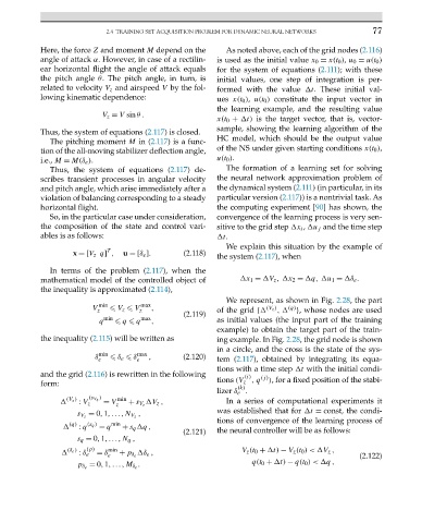
We represent, as shown in Fig. 2.28, the part
V z min V z V z max , (2.119) of the grid { (V z ) , (q) }, whose nodes are used

q min q q max , as initial values (the input part of the training
example) to obtain the target part of the train-
the inequality (2.115) will be written as ing example. In Fig. 2.28, the grid node is shown
in a circle, and the cross is the state of the sys-
δ min δ e δ max , (2.120)
e e tem (2.117), obtained by integrating its equa-
tions with a time step t with the initial condi-
and the grid (2.116) is rewritten in the following (i) (j)
form: tions (V z ,q ), for a fixed position of the stabi-
(k)
lizer δ e .
(V z ) (s V z ) min
= V V z , In a series of computational experiments it
: V z
z + s V z
, was established that for t = const, the condi-
s V z = 0,1,...,N V z
tions of convergence of the learning process of
(q) : q (s q ) = q min + s q q ,
(2.121) the neural controller will be as follows:
s q = 0,1,...,N q ,
(δ e ) (p) = δ min δ e , V z (t 0 + t) − V z (t 0 )< V z ,
: δ e
e + p δ e (2.122)
. q(t 0 + t) − q(t 0 ) < q ,
p δ e = 0,1,...,M δ e