Page 90 - Neural Network Modeling and Identification of Dynamical Systems

78 2. DYNAMIC NEURAL NETWORKS: STRUCTURES AND TRAINING METHODS

2.4.2.4 Assessment of the Volume of the
Training Set With a Direct
Approach to Its Formation
Let us estimate the volume of the training set,
obtained with a direct approach to its formation.
Let us first consider the simplest version of a di-
rect one-step method of forming a training set,
i.e., the one in which the reaction of DS (2.106)
at thetimeinstant t k+1 depends on the values
of the state and control variables (2.105)onlyat
(q)
(V z )
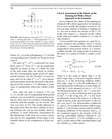
FIGURE 2.28 Fragment of the grid { , } for δ e =
const. ◦ – starting grid node; × –meshtargetpoint; V z , q time instant t k .
is the grid spacing for the state variables V z and q,respec- Let us consider this question on a specific ex-

tively; V , q is the shift of the target point relative to the ample related to the problem, which is solved
z
grid node that spawned it (From [90], used with permission in Section 6.2 (formation of the ANN model of
from Moscow Aviation Institute).
longitudinal short-period motion of a maneu-
verable aircraft). The initial model of motion in
the form of a system of ODEs is written as fol-
where V z , q is the grid spacing (2.121)for the
lows:
corresponding state variables for the given fixed
value δ e . ¯ qS g
˙ α = q − C L (α,q,δ e ) + cosθ,
The grid { (V z ) , (q) }, constructed for some mV V
c
(p) (δ e ) ¯ qS ¯
fixed point δ e from , can be graphically (2.123)
˙ q = C m (α,q,δ e ),
depicted as shown in Fig. 2.29. Here, for each I y
2
of the grid nodes (they are shown as circles), T δ e =−2Tζδ e − δ e + δ e act ,
˙
¨
also the corresponding target points are repre-
sented (crosses). The set (“bundle”) of such im- where α is the angle of attack, deg; θ is the
(p) (δ e ) pitch angle, deg; q is the pitch angular velocity,
ages, each for its value δ e ∈ , gives impor-
deg/sec; δ e is the all-moving stabilizer deflec-
tant information about the structure of the train-
tion angle , deg; C L is the lift coefficient; C m is
ing set for the system (2.117), allowing, in some
pitching moment coefficient; m is mass of the air-
cases, to significantly reduce the volume of this 2
craft, kg; V is the airspeed, m/sec; ¯q = ρV /2 is
set. −1 −2
the dynamic pressure, kg·m sec ; ρ is air den-
Now, after the grid is formed (2.116)(or sity, kg/m ; g is the acceleration due to gravity,
3
(2.121), for the case of longitudinal short-period m/sec ; S is the wing area, m ; ¯c is the mean
2
2
motion), you can build the corresponding train- aerodynamic chord of the wing, m; I y is the mo-
ing set, after which the problem of learning the ment of inertia of the aircraft relative to the lat-
network with the teacher can be solved. This eral axis, kg·m ; the dimensionless coefficients
2
task was done in [90]. The results obtained in C L and C m are nonlinear functions of their argu-
this paper show that the direct method of form- ments; T , ζ are the time constant and the relative
ing training sets can be successfully used for is
damping coefficient of the actuator, and δ e act
problems of small dimension (determined by the command signal to the actuator of the all-
the dimensions of the state and control vectors, moving controllable stabilizer (limited to ±25
and also by the magnitude of the range of ad- deg). In the model (2.123), the variables α, q, δ e ,
missible values of the components of these vec- and δ e are the states of the controlled object, and
˙
tors). the variable δ e act is the control.