Page 137 - Numerical Analysis Using MATLAB and Excel

Cramer’s Rule

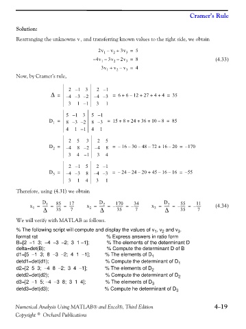
Solution:

Rearranging the unknowns , and transferring known values to the right side, we obtain
v

2v – v + 3v = 5
2
1
3
– 4v – 3v – 2v = 8 (4.33)
2
1
3
3v + v – v = 4
3
1
2
Now, by Cramer’s rule,
2 – 1 3 2 – 1
Δ = – 4 – 3 – 2 – 4 – 3 = 6 + 6 – 12 + 27 + + 4 = 35
4
3 1 – 1 3 1
5 – 1 3 5 – 1
D = 8 – 3 – 2 8 – 3 = 15 + + 24 + 36 + 10 8 = 85
8
–
1
4 1 – 1 4 1
2 5 3 2 5
D = – 4 8 – 2 – 4 8 = – 16 – 30 – 48 – 72 + 16 20 = – 170
–
2
3 4 – 1 3 4
2 – 1 5 2 – 1
D = – 4 – 3 8 – 4 – 3 = – 24 – 24 – 20 + 45 16 16 = – 55
–
–
3
3 1 4 3 1
Therefore, using (4.31) we obtain

D 85 17 D 170 34 D 55 11
2
3
1
x = ------ = ------ = ------ x = ------ = – --------- = – ------ x = ------ = – ------ = – ------ (4.34)
Δ
Δ
3
Δ
2
1
35
7
35
35
7
7
We will verify with MATLAB as follows.
% The following script will compute and display the values of v , v and v .
1 2 3
format rat % Express answers in ratio form
B=[2 −1 3; −4 −3 −2; 3 1 −1]; % The elements of the determinant D
delta=det(B); % Compute the determinant D of B
d1=[5 −1 3; 8 −3 −2; 4 1 −1]; % The elements of D
1
detd1=det(d1); % Compute the determinant of D
1
d2=[2 5 3; −4 8 −2; 3 4 −1]; % The elements of D
2
detd2=det(d2); % Compute the determinant of D
2
d3=[2 −1 5; −4 −3 8; 3 1 4]; % The elements of D
3
detd3=det(d3); % Compute he determinant of D
3
Numerical Analysis Using MATLAB® and Excel®, Third Edition 4−19
Copyright © Orchard Publications