Page 19 - Numerical Analysis Using MATLAB and Excel

Chapter 1 Introduction to MATLAB

Example 1.5
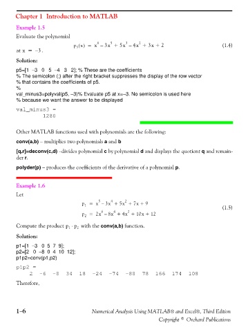
Evaluate the polynomial

3
2
6
5
p x() = x – 3x + 5x – 4x + 3x + 2 (1.4)
5
at x = – . 3
Solution:
p5=[1 −3 0 5 −4 3 2]; % These are the coefficients
% The semicolon (;) after the right bracket suppresses the display of the row vector
% that contains the coefficients of p5.
%
val_minus3=polyval(p5, −3)% Evaluate p5 at x=−3. No semicolon is used here
% because we want the answer to be displayed

val_minus3 =
1280

Other MATLAB functions used with polynomials are the following:

conv(a,b) − multiplies two polynomials a and b
[q,r]=deconv(c,d) −divides polynomial c by polynomial d and displays the quotient q and remain-
der r.

polyder(p) − produces the coefficients of the derivative of a polynomial p.

Example 1.6
Let
4
5
2
p = x – 3x + 5x + 7x + 9 (1.5)
1
4
6
2
p = 2x – 8x + 4x + 10x + 12
2
Compute the product p ⋅ p 2 with the conv(a,b) function.
1
Solution:
p1=[1 −3 0 5 7 9];
p2=[2 0 −8 0 4 10 12];
p1p2=conv(p1,p2)
p1p2 =
2 -6 -8 34 18 -24 -74 -88 78 166 174 108
Therefore,

1−6 Numerical Analysis Using MATLAB® and Excel®, Third Edition
Copyright © Orchard Publications