Page 24 - Numerical Analysis Using MATLAB and Excel

Using MATLAB to Make Plots

2600 2700 2800 2900 3000]; % Use semicolon to suppress display of these numbers
%
z=[39.339 52.789 71.104 97.665 140.437 222.182 436.056....
1014.938 469.830 266.032 187.052 145.751 120.353 103.111....
90.603 81.088 73.588 67.513 62.481 58.240 54.611 51.468....
48.717 46.286 44.122 42.182 40.432 38.845];
Of course, if we want to see the values of w or z or both, we simply type w or z, and we press
<enter>.

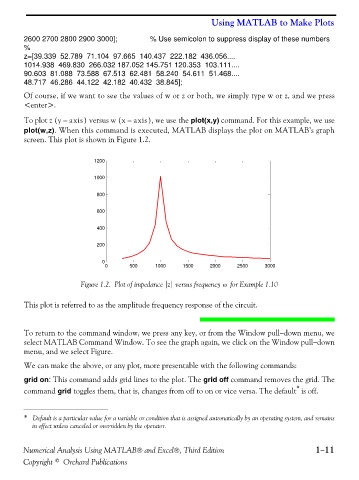
To plot z (y – axis ) versus w (x – axis ), we use the plot(x,y) command. For this example, we use
plot(w,z). When this command is executed, MATLAB displays the plot on MATLAB’s graph
screen. This plot is shown in Figure 1.2.

1200

1000

800

600

400

200

0
0 500 1000 1500 2000 2500 3000
Figure 1.2. Plot of impedance z versus frequency for Example 1.10
ω

This plot is referred to as the amplitude frequency response of the circuit.

To return to the command window, we press any key, or from the Window pull−down menu, we
select MATLAB Command Window. To see the graph again, we click on the Window pull−down
menu, and we select Figure.

We can make the above, or any plot, more presentable with the following commands:

grid on: This command adds grid lines to the plot. The grid off command removes the grid. The
*
command grid toggles them, that is, changes from off to on or vice versa. The default is off.

* Default is a particular value for a variable or condition that is assigned automatically by an operating system, and remains
in effect unless canceled or overridden by the operator.

Numerical Analysis Using MATLAB® and Excel®, Third Edition 1−11
Copyright © Orchard Publications