Page 29 - Numerical Analysis Using MATLAB and Excel

Chapter 1 Introduction to MATLAB

The plots which we have discussed thus far are two−dimensional, that is, they are drawn on two
axes. MATLAB has also a three−dimensional (three−axes) capability and this is discussed next.
The command plot3(x,y,z) plots a line in 3−space through the points whose coordinates are the
x
y
xy
z
z
elements of , , and , where , , and are three vectors of the same length.
The general format is plot3(x ,y ,z ,s ,x ,y ,z ,s ,x ,y ,z ,s ,...) where x , y , and z are vectors
n
n
3 3
n
3
3
1
2 2
2
1 1
2
1
or matrices, and s are strings specifying color, marker symbol, or line style. These strings are the
n
same as those of the two−dimensional plots.
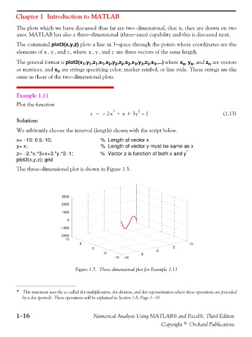
Example 1.11
Plot the function
2
3
z = – 2x ++ 3y – 1 (1.13)
x
Solution:
We arbitrarily choose the interval (length) shown with the script below.
x= −10: 0.5: 10; % Length of vector x
y= x; % Length of vector y must be same as x
*
z= −2.*x.^3+x+3.*y.^2−1; % Vector z is function of both x and y
plot3(x,y,z); grid
The three−dimensional plot is shown in Figure 1.5.

3000
2000

1000
0
-1000
-2000
10
5 10
5
0
0
-5
-5
-10
-10
Figure 1.5. Three dimensional plot for Example 1.11

* This statement uses the so called dot multiplication, dot division, and dot exponentiation where these operations are preceded
by a dot (period). These operations will be explained in Section 1.8, Page 1−19.

1−16 Numerical Analysis Using MATLAB® and Excel®, Third Edition
Copyright © Orchard Publications