Page 31 - Numerical Analysis Using MATLAB and Excel

Chapter 1 Introduction to MATLAB

[R,H]=meshgrid(0: 4, 0: 6); % Creates R and H matrices from vectors r and h
V=(pi .* R .^ 2 .* H) ./ 3; mesh(R, H, V)
xlabel('x−axis, radius r (meters)'); ylabel('y−axis, altitude h (meters)');
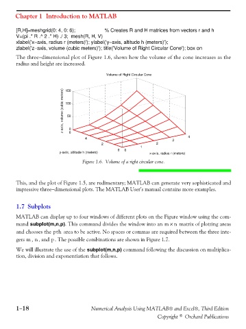
zlabel('z−axis, volume (cubic meters)'); title('Volume of Right Circular Cone'); box on
The three−dimensional plot of Figure 1.6, shows how the volume of the cone increases as the
radius and height are increased.

Volume of Right Circular Cone

z-axis, volume (cubic meters) 100
150

50

6 0
4
4
3
2
2
1
0 0
y-axis, altitude h (meters)
x-axis, radius r (meters)
Figure 1.6. Volume of a right circular cone.

This, and the plot of Figure 1.5, are rudimentary; MATLAB can generate very sophisticated and
impressive three−dimensional plots. The MATLAB User’s manual contains more examples.

1.7 Subplots

MATLAB can display up to four windows of different plots on the Figure window using the com-
mand subplot(m,n,p). This command divides the window into an mn× matrix of plotting areas
and chooses the pth area to be active. No spaces or commas are required between the three inte-
gers mn , and . The possible combinations are shown in Figure 1.7.
,
p
We will illustrate the use of the subplot(m,n,p) command following the discussion on multiplica-
tion, division and exponentiation that follows.

1−18 Numerical Analysis Using MATLAB® and Excel®, Third Edition
Copyright © Orchard Publications