Page 35 - Numerical Analysis Using MATLAB and Excel

Chapter 1 Introduction to MATLAB

Example 1.13
Write the MATLAB script that produces a simple plot for the waveform defined as

2
t
y = f t() = 3e – 4t cos 5t – 2e – 3t sin 2t + ------------- (1.17)
t + 1
in the 0t5 seconds interval.
≤≤
Solution:

The MATLAB script for this example is as follows:

t=0: 0.01: 5; % Define t−axis in 0.01 increments
y=3 .* exp(−4 .* t) .* cos(5 .* t)−2 .* exp(−3 .* t) .* sin(2 .* t) + t .^2 ./ (t+1);
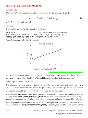
plot(t,y); grid; xlabel('t'); ylabel('y=f(t)'); title('Plot for Example 1.13')
Figure 1.8 shows the plot for this example.

Plot for Example 1.13
6

4
y=f(t) 2

0

-2
0 1 2 3 4 5
t
Figure 1.8. Plot for Example 1.13

Had we, in the example above, defined the time interval starting with a negative value equal to or
less than 1– , say as 3t3≤≤– , MATLAB would have displayed the following message:

Warning: Divide by zero.
This is because the last term (the rational fraction) of the given expression, is divided by zero when
t = – 1 . To avoid division by zero, we use the special MATLAB function eps, which is a number

approximately equal to 2.2 × 10 – 16 . It will be used with the next example.

The command axis([xmin xmax ymin ymax]) scales the current plot to the values specified by
the arguments xmin, xmax, ymin and ymax. There are no commas between these four argu-
ments. This command must be placed after the plot command and must be repeated for each plot.

The following example illustrates the use of the dot multiplication, division, and exponentiation,
the eps number, the axis([xmin xmax ymin ymax]) command, and also MATLAB’s capability of

1−22 Numerical Analysis Using MATLAB® and Excel®, Third Edition
Copyright © Orchard Publications