Page 37 - Numerical Analysis Using MATLAB and Excel

Chapter 1 Introduction to MATLAB

The next example illustrates MATLAB’s capabilities with imaginary numbers. We will introduce
the real(z) and imag(z) functions which display the real and imaginary parts of the complex quan-
tity z = x + iy, the abs(z), and the angle(z) functions that compute the absolute value (magni-
–
tude) and phase angle of the complex quantity z = x + iy = r θ . We will also use the
polar(theta,r) function that produces a plot in polar coordinates, where r is the magnitude, theta
is the angle in radians, and the round(n) function that rounds a number to its nearest integer.

Example 1.15

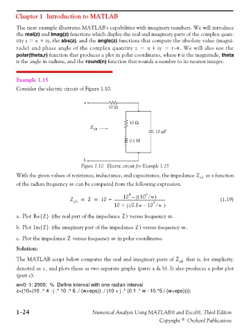
Consider the electric circuit of Figure 1.10.

a
10 Ω

10 Ω
Z ab
10 μF

0.1 H

b
Figure 1.10. Electric circuit for Example 1.15

With the given values of resistance, inductance, and capacitance, the impedance Z ab as a function
ω
of the radian frequency can be computed from the following expression.
6
4
(
)
10 –
w
j10 ⁄
Z ab = Z = 10 + -------------------------------------------------------- (1.19)
5
(
10 + j 0.1w – 10 ⁄ w )
ω
a. Plot Re Z{} (the real part of the impedance ) versus frequency .
Z
ω
b. Plot Im Z{} (the imaginary part of the impedance ) versus frequency .
Z
ω
Z
c. Plot the impedance versus frequency in polar coordinates.
Solution:
The MATLAB script below computes the real and imaginary parts of Z ab that is, for simplicity,
z
denoted as , and plots these as two separate graphs (parts a & b). It also produces a polar plot
(part c).
w=0: 1: 2000; % Define interval with one radian interval
z=(10+(10 .^ 4 −j .* 10 .^ 6 ./ (w+eps)) ./ (10 + j .* (0.1 .* w −10.^5./ (w+eps))));

1−24 Numerical Analysis Using MATLAB® and Excel®, Third Edition
Copyright © Orchard Publications