Page 41 - Numerical Analysis Using MATLAB and Excel

Chapter 1 Introduction to MATLAB

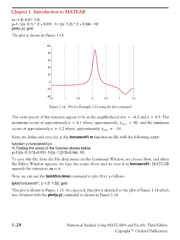
x=−1.5: 0.01: 1.5;
y=1./ ((x−0.1).^ 2 + 0.01) −1./ ((x−1.2).^ 2 + 0.04) −10;
plot(x,y); grid
The plot is shown in Figure 1.14.

100

80
60

40

20

0
-20

-40
-1.5 -1 -0.5 0 0.5 1 1.5
Figure 1.14. Plot for Example 1.16 using the plot command

The roots (zeros) of this function appear to be in the neighborhood of x = – 0.2 and x = 0.3 . The
maximum occurs at approximately x = 0.1 where, approximately, y max = 90 , and the minimum
occurs at approximately x = 1.2 where, approximately, y min = – 34 .

Next, we define and save f(x) as the funczero01.m function m−file with the following script:

function y=funczero01(x)
% Finding the zeros of the function shown below
y=1/((x−0.1)^2+0.01)−1/((x−1.2)^2+0.04)−10;
To save this file, from the File drop menu on the Command Window, we choose New, and when
the Editor Window appears, we type the script above and we save it as funczero01. MATLAB
appends the extension .m to it.

Now, we can use the fplot(fcn,lims) command to plot fx() as follows:

fplot('funczero01', [−1.5 1.5]); grid
This plot is shown in Figure 1.15. As expected, this plot is identical to the plot of Figure 1.14 which
was obtained with the plot(x,y) command as shown in Figure 1.14.

1−28 Numerical Analysis Using MATLAB® and Excel®, Third Edition
Copyright © Orchard Publications