Page 43 - Numerical Analysis Using MATLAB and Excel

Chapter 1 Introduction to MATLAB

solve(zmin)
is executed, MATLAB displays a very long expression which when copied at the command prompt
and executed, produces the following:

ans =
0.6585 + 0.3437i
ans =
0.6585 - 0.3437i
ans =
1.2012
x
y
The real value 1.2012 above is the value of at which the function has its minimum value as
we observe also in the plot of Figure 1.15.
To find the value of y corresponding to this value of x, we substitute it into fx() , that is,

x=1.2012; ymin=1 / ((x−0.1) ^ 2 + 0.01) −1 / ((x−1.2) ^ 2 + 0.04) −10
ymin = -34.1812
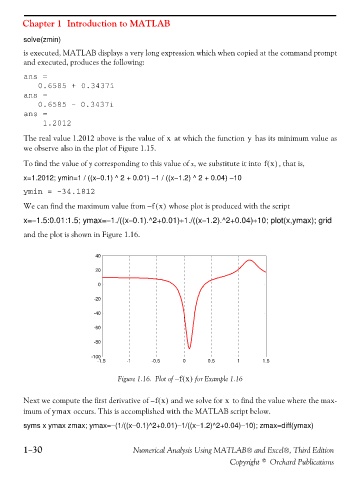
We can find the maximum value from fx() whose plot is produced with the script
–

x=−1.5:0.01:1.5; ymax=−1./((x−0.1).^2+0.01)+1./((x−1.2).^2+0.04)+10; plot(x,ymax); grid
and the plot is shown in Figure 1.16.

40

20
0

-20

-40
-60

-80

-100
-1.5 -1 -0.5 0 0.5 1 1.5
Figure 1.16. Plot of fx() for Example 1.16
–

Next we compute the first derivative of fx() and we solve for to find the value where the max-
x
–
imum of ymax occurs. This is accomplished with the MATLAB script below.

syms x ymax zmax; ymax=−(1/((x−0.1)^2+0.01)−1/((x−1.2)^2+0.04)−10); zmax=diff(ymax)

1−30 Numerical Analysis Using MATLAB® and Excel®, Third Edition
Copyright © Orchard Publications