Page 27 - Numerical Analysis Using MATLAB and Excel

Chapter 1 Introduction to MATLAB

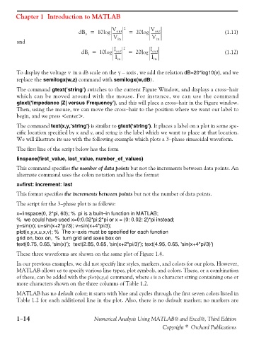
dB = 10log V out 2 = 20log V out (1.11)
----------
----------
v
and V in V in
dB = 10log I -------- 2 = 20log I -------- (1.12)
out
out
i
I in I in
To display the voltage in a dB scale on the v y – axis , we add the relation dB=20*log10(v), and we
replace the semilogx(w,z) command with semilogx(w,dB).
The command gtext(‘string’) switches to the current Figure Window, and displays a cross−hair
which can be moved around with the mouse. For instance, we can use the command
gtext(‘Impedance |Z| versus Frequency’), and this will place a cross−hair in the Figure window.
Then, using the mouse, we can move the cross−hair to the position where we want our label to
begin, and we press <enter>.

The command text(x,y,’string’) is similar to gtext(‘string’). It places a label on a plot in some spe-
cific location specified by x and y, and string is the label which we want to place at that location.
We will illustrate its use with the following example which plots a 3−phase sinusoidal waveform.

The first line of the script below has the form

linspace(first_value, last_value, number_of_values)
This command specifies the number of data points but not the increments between data points. An
alternate command uses the colon notation and has the format
x=first: increment: last

This format specifies the increments between points but not the number of data points.

The script for the 3−phase plot is as follows:

x=linspace(0, 2*pi, 60); % pi is a built−in function in MATLAB;
% we could have used x=0:0.02*pi:2*pi or x = (0: 0.02: 2)*pi instead;
y=sin(x); u=sin(x+2*pi/3); v=sin(x+4*pi/3);
plot(x,y,x,u,x,v); % The x−axis must be specified for each function
grid on, box on, % turn grid and axes box on
text(0.75, 0.65, 'sin(x)'); text(2.85, 0.65, 'sin(x+2*pi/3)'); text(4.95, 0.65, 'sin(x+4*pi/3)')
These three waveforms are shown on the same plot of Figure 1.4.
In our previous examples, we did not specify line styles, markers, and colors for our plots. However,
MATLAB allows us to specify various line types, plot symbols, and colors. These, or a combination
of these, can be added with the plot(x,y,s) command, where s is a character string containing one or
more characters shown on the three columns of Table 1.2.
MATLAB has no default color; it starts with blue and cycles through the first seven colors listed in
Table 1.2 for each additional line in the plot. Also, there is no default marker; no markers are

1−14 Numerical Analysis Using MATLAB® and Excel®, Third Edition
Copyright © Orchard Publications